my_function_name <- function(parameter1, parameter2="default value"){
  retVal <- parameter1 + 1
  return(retVal)
}R & Statistics — Master Notes
A ground-up reference for learning R and applied statistics
Below are notes I assembled over the course of grad school both for tutoring and personal reference. They cover the basics of R and applied statistics for social science assuming no prior programming experience and build up to estimating and diagnosing regression models. Code blocks show real output; in the HTML version a few examples are live and editable, so you can change the code and re-run it right in your browser. A PDF version is also available.
1 R Studio Tips
1.1 Keyboard Shortcuts
ALT + SHIFT + K => shows all keyboard shortcuts
CMD + ALT + I => insert new code chunk
CMD + ENTER => run the line of code your cursor is currently on or what’s highlighted
CMD + SHIFT + ENTER => run current code chunk
CMD + SHIFT + M => insert pipe operator (%>%)
ALT + O => collapse all chunks
1.2 Working Directory, Environment, and Data Storing
The following can be typed in the console or a code chunk and run:
install.packages("package_name") => install or update a package
library(package_name) => load an installed package
?function_name => opens the documentation for a function
typeof(object_name) => gives the type of an object
getwd() => get the current working directory
setwd("your/directory/path") => set the working directory (don’t do this if you’re working inside a project)
rm(object_name) => remove an object from the R environment
saveRDS(example_data, "example_data.rds") => save a single R object to a file
example_data <- readRDS("example_data.rds") => read in a saved R object and store it as a variable
save.image(file="my_environment.RData") => save the environment into a file
load("my_environment.RData") => load a saved environment
2 Using Functions
2.1 Custom Functions
To write a custom function you generally need 3 things: a name, parameters, and a return value.
Parameters are variables that exist only within the scope of the function, they will not show up in your environment or be able to be used outside the function.
Parameters can either be left without a default value (like parameter1 below) or assigned a default value (like parameter2 below) they will take on if you don’t pass an argument to them.
When you write custom functions, if you don’t use return() the evaluation of the last line of code inside the function is returned. For example the below will behave the same as my_function_name() above:
my_other_function_name <- function(parameter1, parameter2="default value"){
  parameter1 + 1
}
To call a function we type its name followed by parentheses. Within the parentheses we can pass arguments–arguments are values we assign to parameters.
# note we don't need to pass an argument to parameter2 (but we can if we want)
my_function_name(parameter1=27)
[1] 28Try it yourself. Edit the function body or the argument, then press Run Code. What happens if you remove the return()?
2.2 Existing Functions
There are two classes of built-in functions: base R functions and functions from libraries.
These functions operate exactly the same as custom functions you write, they take in parameters and return a value.
2.2.1 Built-in
These functions can be used without loading any libraries, they include the most basic functions (e.g. sum(), seq(), data.frame(), plot(), hist()) as well as more advanced statistical functions (e.g. lm(), t.test(), rnorm()).
2.2.2 Functions from Libraries
These functions exist in libraries (AKA packages) that must be installed (once per machine) and loaded (once per R session) before the function can be called.
To install (or update) a library use install.packages("package_name"). To load a library use library(package_name).
Conflicts
When you load a library you may sometimes see a conflict warning. This means that a function in the library has the same name as one already in the environment (i.e. built-in, from another loaded library, or custom). Generally the order the functions are loaded determines precedence. For example, if I load tidyverse and then MASS, both libraries have a function called select(). dplyr::select() (dplyr is one of the packages included in tidyverse) will be masked by MASS::select() so when you use select() in your code it will by default use the function from MASS.
# install.packages("tidyverse")
library(tidyverse)
# install.packages("MASS")
library(MASS)
To use the masked version of select() you need to tell R which library (also called namespace) it’s from using a double colon i.e. dplyr::select().
If using the namespace constantly is too annoying (or you would have to retrofit code to work after a new package is loaded) the conflicted library offers another solution. The conflict_prefer() function allows you to tell R which version of select() (or any other function) to default to:
# install.packages("conflicted")
library(conflicted)

# Tell R to use dplyr::select() by default
conflict_prefer(name="select", winner="dplyr")
The library also provides the conflict_prefer_all() function which will tell R to prefer all the functions in one library over functions of the same name in another:
# Tell R to always defer to dplyr for functions of the same name in
# MASS and dplyr
conflict_prefer_all(winner="dplyr", losers="MASS")
3 Operators
Operators are symbols that effectively do something a function would normally do, for example:
1 + 2[1] 3# is the same as
sum(1, 2)[1] 3Click here for a comprehensive list of base R operators
Try it yourself. This is real R running in your browser. Change the numbers, try *, /, ^ (power), or %% (remainder), then press Run Code.
3.1 Logical operators
Use these to subset data frames, vectors, etc. based on conditions.
# logical AND
T & F
[1] FALSE# logical OR
T | F[1] TRUE# logical NOT
!TRUE[1] FALSE# check if element is in a vector/list
1 %in% c(2:4)[1] FALSE3.2 Pipe operator
Beyond the base R operators, tidyverse gives the piping operator, %>%. This serves as a “pipe”, think of it as feeding an object on its left side into the function as an argument on its right side.
library(tidyverse)

sum(1, 2)
[1] 3# is equivalent to
1 %>% sum(2)[1] 3This is most useful when working with data frames in the tidyverse, it avoids having a million nested parentheses and gives you a more sequential way of manipulating data so it’s easier to know what’s going on and make changes.
social <- read.csv("social.csv")

# Suppose we want to do some cleaning to the above data.

## Without piping
social2 <- summarize(social, group_by(social, mutate(
  select(social, sex, primary2004, primary2006),
             primarysum=primary2004 + primary2006), sex),
             primarysum=sum(primarysum))

## With piping
library(tidyverse)

social2 <- social %>% select(sex, primary2004, primary2006) %>%
  mutate(primarysum=primary2004 + primary2006) %>%
  group_by(sex) %>%
  summarize(primarysum=sum(primarysum))
4 Variable Types
4.1 Value Types
R has a few kinds of values that can be stored in variables:
4.1.1 Integer
An integer, a whole number with no decimals. Note that R stores numeric literals as doubles by default, so to actually get the integer type you append an L.
var <- -24L

typeof(var)
[1] "integer"4.1.2 Numeric
A (real) number, also known as a double
var <- 255.758

typeof(var)
[1] "double"# Can also use scientific notation
var2 <- 5e-4
typeof(var2)[1] "double"4.1.3 Character
One or more characters, AKA a string or character vector if more than one character
var <- "n"

typeof(var)
[1] "character"var2 <- "noodle24"
typeof(var2)[1] "character"4.1.4 Logical
True or false, AKA a boolean. In certain circumstances R will interpret a 0 as false and 1 as true.
# Note: you can use TRUE or T, FALSE or F
var <- TRUE

typeof(var)
[1] "logical"var2 <- F
typeof(var2)[1] "logical"4.1.5 Complex
Complex numbers, rarely used for our purposes
var <- 10 + 5i

typeof(var)
[1] "complex"Try it yourself. Assign different values and check their type with typeof(). Try a decimal, a word in quotes, TRUE, or 5L (the L forces an integer).
4.2 Data Structures
R has several data structures for storing multiple values:
4.2.1 Vectors
A list of values of the same type i.e. you can’t store a numeric and a string in the same vector, for that use a list
vec <- c(4, 5, 7, -12)

# access values from a vector with hard brackets and the index of the desired
# value
vec[3]
[1] 7# you can also access multiple values by putting a vector of indexes in the
# brackets
vec[c(1,3,4)][1] 4 7 -12# get the length of a vector with the length() function
length(vec)[1] 4# append to a vector by nesting it inside of another vector
# we have to effectively create a new vector to do this because vectors are not
# dynamic (can't change length)
vec2 <- c(vec, 45, 23)
vec2[1] 4 5 7 -12 45 23# you can operate on a numeric vector like you would a single numeric
# i.e. you can double all the values in a vector as follows:
2 * vec2[1] 8 10 14 -24 90 46# To easily make a sequence of numbers increasing or decreasing by 1 use a colon:
1:10 [1] 1 2 3 4 5 6 7 8 9 10-4.5:-10[1] -4.5 -5.5 -6.5 -7.5 -8.5 -9.5# To make a sequence increasing or decreasing by something other than 1 use seq():
seq(1, 10, by=2)[1] 1 3 5 7 9# To make a vector repeating one or more values use rep():
rep(1, 5)[1] 1 1 1 1 1rep(1:4, 5) [1] 1 2 3 4 1 2 3 4 1 2 3 4 1 2 3 4 1 2 3 4# To reverse a vector use rev():
rev(c(1:10)) [1] 10 9 8 7 6 5 4 3 2 1Vectors can have their elements named so you can more easily access them.
named_vec <- c("thing1"=1, "thing2"=2)
# can also omit quotes if there's no spaces in the string: c(thing1=1, thing2=2)

# now you can access the elements by their name (has to be in quotes here):
named_vec["thing1"]
thing1
1 # You can assign names to an unnamed vector with the names() function:
vec <- 1:3
names(vec) <- c("thing1", "thing2", "thing3")
vecthing1 thing2 thing3
1 2 3 Try it yourself. Build a vector, pull out elements by index, and do math on the whole thing at once. Try rev(vec), sum(vec), or vec[c(1, 3)].
4.2.2 Lists
Lists are like vectors but they can hold any kind of object in them, even other lists or vectors. Unlike vectors, lists are dynamic so an existing list can have its size changed.
my_list <- list(24, c("this", "is", "a", "vector"), 0.235)

# you can access elements like you would for a vector with DOUBLE hard brackets:
my_list[[2]]
[1] "this" "is" "a" "vector"# and you can get the length with the length() function as well:
length(my_list)[1] 3# nested lists are useful in a lot of scenarios but can be more confusing to
# navigate
# This list is 2-dimensional, meaning each element is itself a list, its
# structure is similar to a matrix
nested_list <- list(list(1, 2, 3), list("some", "elements"), list(0, 0, NA))
# Because it's two dimensional we have two "layers" of indexes
# To get the first element (a list) we do:
nested_list[[1]][[1]]
[1] 1
[[2]]
[1] 2
[[3]]
[1] 3# But if we wanted to get the second element of the first nested list we would do:
nested_list[[1]][[2]][1] 2# If we want to remove the nested structure and "flatten" the list to be
# one-dimensional we can use unlist():
unlist(nested_list)[1] "1" "2" "3" "some" "elements" "0" "0"
[8] NA # To append to a list we assign the new element to n+1th index:
nested_list[[length(nested_list)+1]] <- "something we want to add"
# Like vectors, lists can also have named elements:
named_nested_list <- list(thing1=list(1, 2, 3), thing2=list("some", "elements"),
thing3=list(0, 0, NA))
named_nested_list[["thing1"]][[1]]
[1] 1
[[2]]
[1] 2
[[3]]
[1] 3# OR (note this doesn't work for vectors)
named_nested_list$thing1[[1]]
[1] 1
[[2]]
[1] 2
[[3]]
[1] 34.2.3 Matrices
Matrices are essentially just 2D nested lists whose elements must all be of the same type. They’re really only useful if you need to do linear algebra or need your code to be very efficient.
# To create a matrix we need to specify:
# data: a list or vector with the values we want in the matrix
# ncol: the number of columns
# nrow: the number of rows
my_matrix <- matrix(data=1:25, nrow=5, ncol=5)

# To access an element from a matrix we use brackets with a row index and a
# column index inside:
my_matrix[1,4] # get the element in row 1, column 4
[1] 16my_matrix[2,] # get all elements in row 2[1] 2 7 12 17 22my_matrix[,3] # get all elements in column 3[1] 11 12 13 14 15my_matrix[1:3, 2] # get elements in rows 1, 2, and 3 from column 2[1] 6 7 8# You can operate on matrices in a number of ways:
# add, subtract, multiply, divide by a scalar
my_matrix * 2 [,1] [,2] [,3] [,4] [,5]
[1,] 2 12 22 32 42
[2,] 4 14 24 34 44
[3,] 6 16 26 36 46
[4,] 8 18 28 38 48
[5,] 10 20 30 40 50# perform matrix multiplication
my_other_matrix <- matrix(data=runif(25), nrow=5, ncol=5)
my_matrix %*% my_other_matrix [,1] [,2] [,3] [,4] [,5]
[1,] 33.02001 33.07953 21.64650 36.08592 23.21750
[2,] 36.41297 36.35906 23.18477 39.16852 25.77457
[3,] 39.80593 39.63860 24.72303 42.25112 28.33164
[4,] 43.19890 42.91813 26.26129 45.33372 30.88872
[5,] 46.59186 46.19767 27.79955 48.41632 33.44579# transpose the matrix
t(my_matrix) [,1] [,2] [,3] [,4] [,5]
[1,] 1 2 3 4 5
[2,] 6 7 8 9 10
[3,] 11 12 13 14 15
[4,] 16 17 18 19 20
[5,] 21 22 23 24 25# invert the matrix
solve(my_other_matrix) [,1] [,2] [,3] [,4] [,5]
[1,] 0.8102402 1.3180839 -0.1376843 -1.39285342 0.6749147
[2,] 0.2381355 -1.7391510 2.3586604 -0.41645291 -1.7989859
[3,] -0.2064798 -0.7201478 -0.2255952 0.07310128 2.3851777
[4,] -1.1206150 0.6517534 -0.4732190 1.33588055 -0.2407698
[5,] 0.4856873 0.5201559 -1.7451128 1.11895042 0.65819164.2.4 Data Frames
Data frames are, in a technical sense, a list of named vectors. Each column contains values that must be all the same type, i.e. we can’t have one entry be a numeric and another be a string in a column.
The main advantages of data frames over, say, a list of lists or a matrix, is how RStudio lets you view them in a nice format and all the data manipulation functions in base R and tidyverse.
Creating Data Frames
# From scratch:
df <- data.frame(my_column=c(2, 4, 5, 6),
                 my_other_column=rep(c("hello", "world"), 2))

# From a named list of vectors:
list_of_vecs <- list(element1=1:4, element2=rep(c("hello", "world"), 2))

df <- as.data.frame(list_of_vecs)

# By reading in data (most any function that does this returns the data as a
# data frame):
df <- read.csv("social.csv")

# By row binding (requires tidyverse):
library(tidyverse)

row1 <- list(element1=5, element2="blah")
row2 <- list(element1=10, element2="blah blah")

df <- bind_rows(row1, row2)

# By column binding (base R; note cbind() returns a matrix, so wrap it in
# as.data.frame() if you want a data frame):
col1 <- 1:20
col2 <- seq(100, 500, length.out=20)

df <- as.data.frame(cbind(col1, col2))
Accessing Data Frame Values
# note: head gets the first 6 rows of a data frame, I use it here so the below
# output is more readable
df <- head(read.csv("social.csv"))

# By index (the same as we would a matrix):

## Access row 1, column 2's element:
df[1,2]
[1] 1941## Access all of row 1:
df[1,] sex yearofbirth primary2004 messages primary2006 hhsize
1 male 1941 0 Civic Duty 0 2## Access all of column 2:
df[,2][1] 1941 1947 1951 1950 1982 1981## Access rows 1, 2, and 3 of column 2:
df[1:3,2][1] 1941 1947 1951# By column name
df$yearofbirth[1] 1941 1947 1951 1950 1982 1981## OR equivalently
df[,"yearofbirth"][1] 1941 1947 1951 1950 1982 1981Manipulating Data Frames
In base R you can use the subset() function to subset a data frame based on a logical test or selection of columns:
# keep only the rows where sex = "male"
subset(df, sex=="male")
sex yearofbirth primary2004 messages primary2006 hhsize
1 male 1941 0 Civic Duty 0 2
3 male 1951 0 Hawthorne 1 3
6 male 1981 0 Control 0 3# keep only rows where sex = "male" and yearofbirth < 1980
subset(df, sex=="male" & yearofbirth<1980) sex yearofbirth primary2004 messages primary2006 hhsize
1 male 1941 0 Civic Duty 0 2
3 male 1951 0 Hawthorne 1 3# keep only the columns from sex through primary2004
subset(df, select=sex:primary2004) sex yearofbirth primary2004
1 male 1941 0
2 female 1947 0
3 male 1951 0
4 female 1950 0
5 female 1982 0
6 male 1981 0In tidyverse there are a gazillion functions for manipulating data frames, I go over some of the most commonly used below. You can go to Help > Cheat Sheets > Data transformation with dplyr in RStudio for a more comprehensive reference.
Some more commonly used tidyverse functions:
library(tidyverse)
social <- read.csv("social.csv")

# Select certain columns (the order you select them is the order they will be
# in the data frame from here on out)
social <- social %>% select(sex, primary2004, messages, yearofbirth, hhsize)

# Create a new column or change an existing one
social <- social %>% mutate(sex_numeric = ifelse(sex=="male", 1, 0))

# Create a new column case-by-case
social <- social %>% mutate(sex_numeric = case_when(
  sex=="male" ~ 1,
  sex=="female" ~ 0,
  T ~ NA_integer_ # This catches cases we didn't consider, always include
))                # in a case_when with the NA type corresponding to the other
                  # values in the column

# Create a new column containing row numbers (useful for making an ID variable)
social <- social %>% mutate(id=row_number())

# Rename existing columns, newname = oldname
social <- social %>% rename(yearborn=yearofbirth, householdsize=hhsize)

# Group observations by one or more variables
social <- social %>% group_by(sex, householdsize)

# Summarize by group, e.g. getting the average by sex
social %>% group_by(sex) %>% summarize(avg_householdsize = mean(householdsize))
# A tibble: 2 × 2
sex avg_householdsize
<chr> <dbl>
1 female 2.17
2 male 2.20# Get the number of observations in each group
social <- social %>% group_by(sex) %>% mutate(num_of_sex=n())
# View the entire data frame in a separate tab, useful when you're not ready to
# save a data frame but just want to see how it looks after some manipulation
# (only works in interactive RStudio, so it's commented out here)
# social %>% View()Pivots
Pivoting data frames from long to wide or vice versa is also very useful
Wide to long:
social <- read.csv("social.csv")
# Take the selected columns (primary2004 and primary2006) and combine their
# values into one column (values) and label the values in another column
# (primaryyear)
# This is most useful for plotting facets, i.e. if we wanted a facet
# (individual plot) for each primary year we would use facet_wrap(~primaryyear)
social_longer <- social %>% pivot_longer(c(primary2004, primary2006),
                        names_to="primaryyear",
                        values_to="value")

head(social_longer)
# A tibble: 6 × 6
sex yearofbirth messages hhsize primaryyear value
<chr> <int> <chr> <int> <chr> <int>
1 male 1941 Civic Duty 2 primary2004 0
2 male 1941 Civic Duty 2 primary2006 0
3 female 1947 Civic Duty 2 primary2004 0
4 female 1947 Civic Duty 2 primary2006 0
5 male 1951 Hawthorne 3 primary2004 0
6 male 1951 Hawthorne 3 primary2006 1# Take new column names from one column (primaryyear) and put the values from
# corresponding values in another column into them (value)
# Note this reverses the pivot_longer we did above and leaves us with our
# original dataframe
social_longer %>% pivot_wider(names_from=primaryyear, values_from=value) %>%
head() # A tibble: 6 × 6
sex yearofbirth messages hhsize primary2004 primary2006
<chr> <int> <chr> <int> <list> <list>
1 male 1941 Civic Duty 2 <int [175]> <int [175]>
2 female 1947 Civic Duty 2 <int [317]> <int [317]>
3 male 1951 Hawthorne 3 <int [87]> <int [87]>
4 female 1950 Hawthorne 3 <int [91]> <int [91]>
5 female 1982 Hawthorne 3 <int [105]> <int [105]>
6 male 1981 Control 3 <int [421]> <int [421]>A common scenario where you’ll pivot data longer is when you want to have separate panels (AKA facets) within the same plot.
social <- read.csv("social.csv")

social %>% pivot_longer(c(primary2004, primary2006),
                        names_to="primaryyear",
                        values_to="value") %>%
  ggplot(aes(x=hhsize, y=value)) +
  geom_point() +
  theme_bw() +
  facet_wrap(~primaryyear)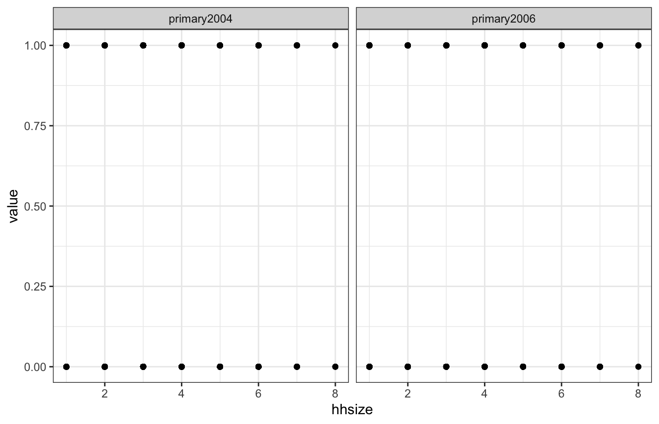
Joins
Joins combine two data frames by matching rows on one or more shared key columns. The four you’ll reach for most, all from dplyr:
inner_join()— keep only rows that have a match in both data framesleft_join()— keep all rows from the left data frame, filling unmatched right-hand columns withNA(this is the one you’ll use most often)right_join()— the mirror image: keep all rows from the rightfull_join()— keep all rows from both
Each takes a by= argument naming the key column(s) to match on; omit it and dplyr will join on every column the two data frames share.
Click here for examples and animations of the different types of joins
5 Plotting
5.1 Base R
Base R plots use a single function call, i.e. to plot(), to generate a plot. You pass additional arguments to customize the plot.
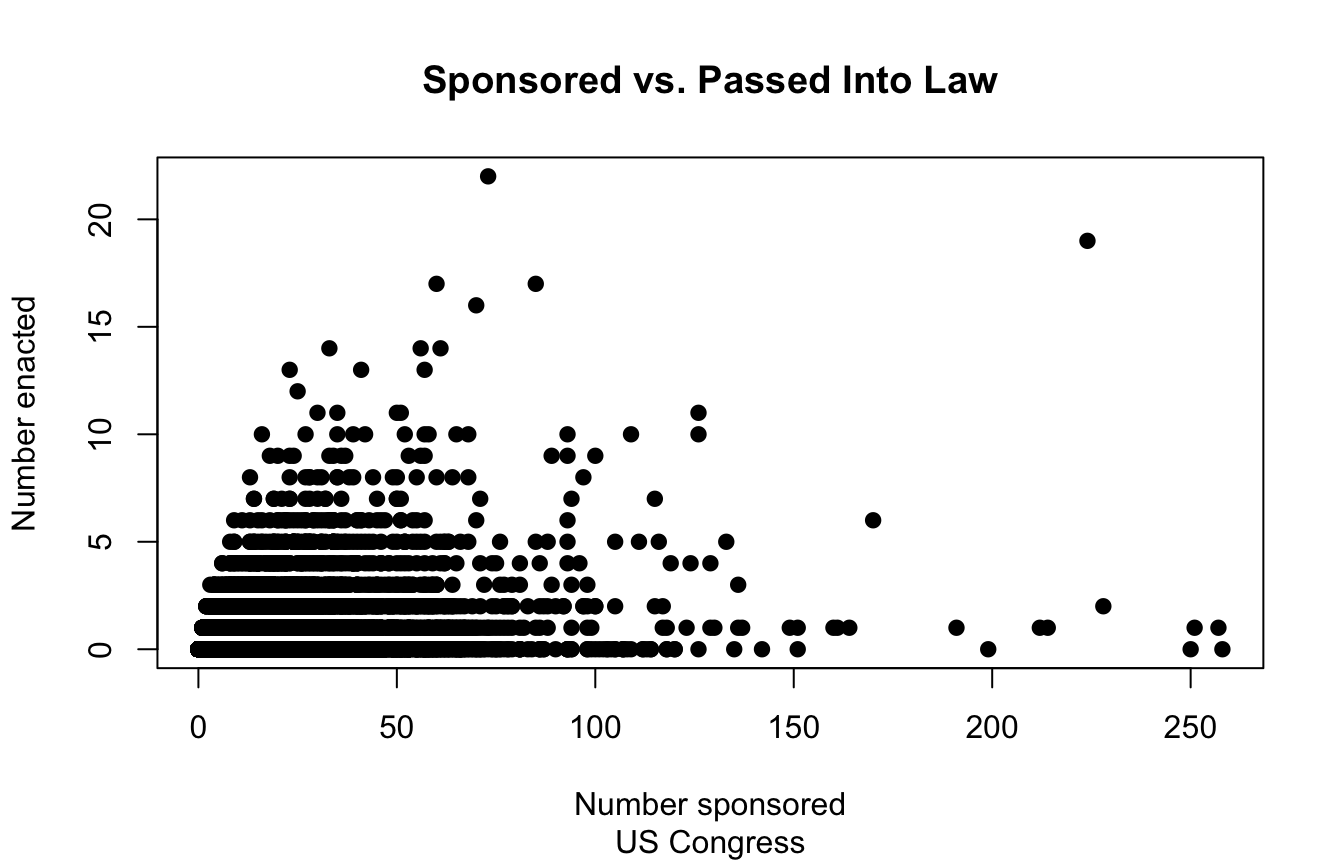
library(readxl)
CEL <- read_excel("CELHouse.xls")

# Scatter plot
plot(x=CEL$sponsored_total, y=CEL$law_total,
     main="Sponsored vs. Passed Into Law", # Set the title
     sub="US Congress", # Set the subtitle
     xlab="Number sponsored", ylab="Number enacted", # Set axis labels
     pch=19 # Set the point shape
     )
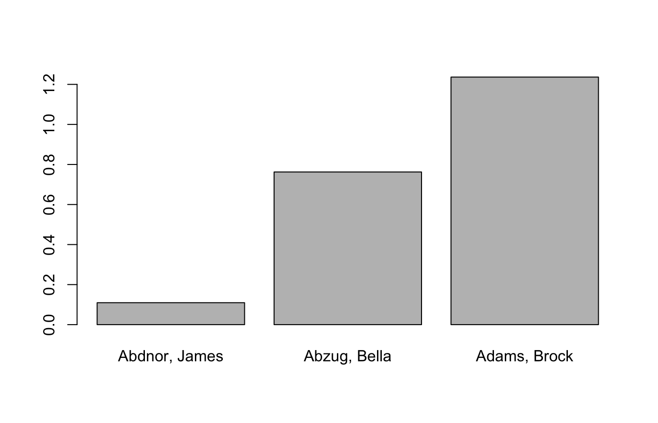
# Bar plot
barplot(CEL$les[1:3], # Plot a bar for each of the first 3 values of les
        names.arg=CEL$name[1:3] # Label bars with names
        )
# Histogram
hist(CEL$congress)

# Multi-panel plots
par(mfrow=c(1,2)) # Have one row, two columns of plots
hist(CEL$congress)
hist(CEL$democrat)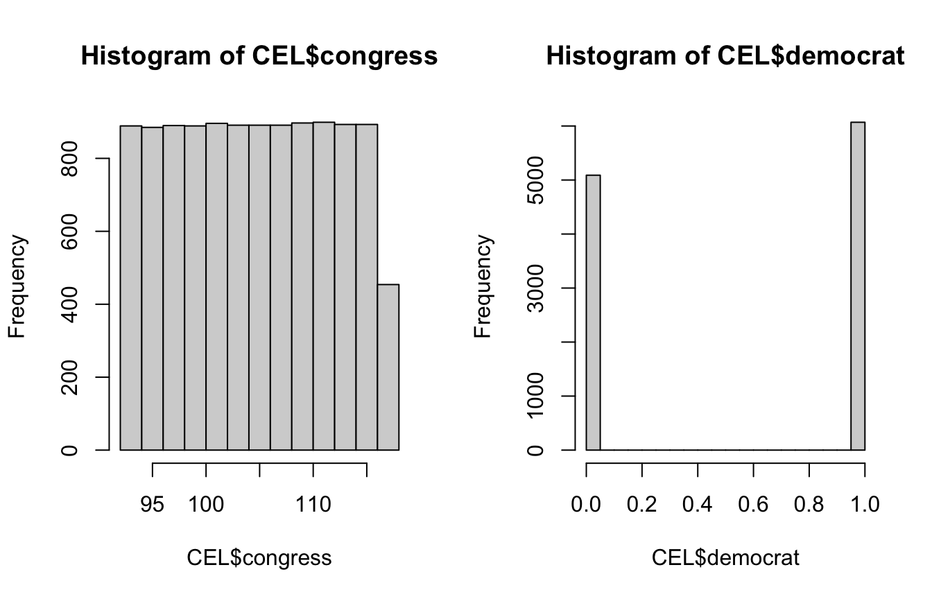
Try it yourself. Base R plots render right in the browser. Change n, the mean, or the number of breaks and re-run to see the histogram update.
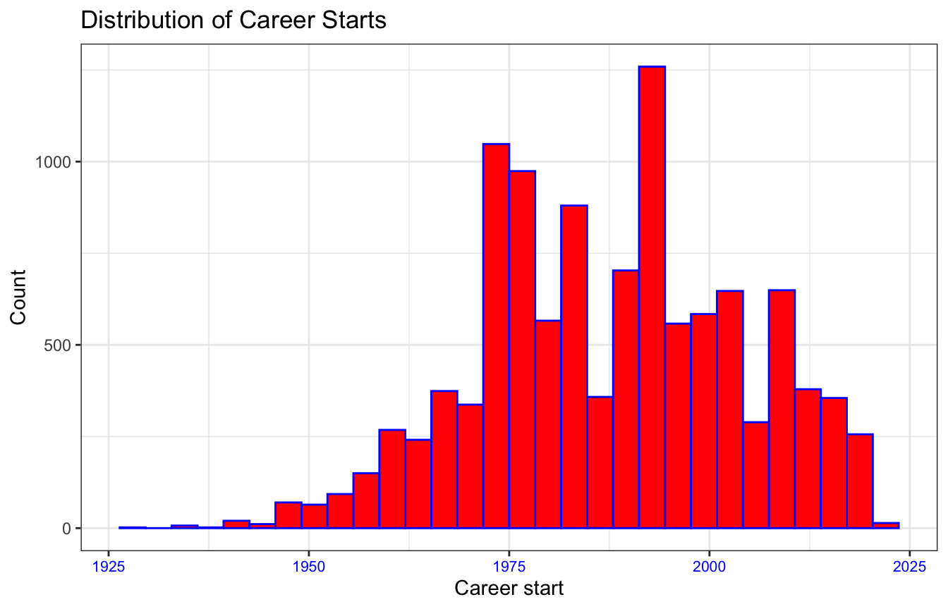
5.2 ggplot2
ggplot uses a different structure for generating plots that allows for more customization. The thought process is similar to piping–you sequentially add onto the plot with additional function calls.
library(readxl)
CEL <- read_excel("CELHouse.xls")

library(tidyverse)
# We always start wtih a call to ggplot() to which we pass a data frame
# and aesthetic mappings (i.e. what data frame column is our x, what column
# determines point color, etc.)
# Note we could also pipe our data frame into ggplot(), maybe doing some
# manipulation before plotting:
#   CEL %>% mutate(years_since_start=2024-career_start) %>%
#   ggplot(aes(x=years_since_start))
ggplot(data = CEL, mapping = aes(x=career_start)) + # Use + to add layers
  geom_histogram(fill="red", color="blue") + # geom_whatever layers determine
                                             # the type of plot and lets you
                                             # customize it
  labs(x="Career start", y="Count",
       title="Distribution of Career Starts") + # Set labels and title
  theme_bw() + # theme_whatever sets the theme to a default of your choosing
  theme( # theme lets you edit the theme, always add AFTER setting a default
         # theme
    # You can edit almost anything in here but some common things:
    axis.text.x = element_text(size=8, color="blue"), # Change format of axis
                                                     # labels
    legend.position = "none", # Remove the legend
  )
# Common types of plots:
#   geom_point() - scatter plot
#   geom_errorbar() - error bars for points
#   geom_line() - line plot
#   geom_smooth() - curved line/fit line plot
#   geom_bar() - bar plot
#   geom_density() - probability density plot
#   geom_boxplot() - box plot


# Common aesthetics (i.e. things you use in the geom_ functions to tweak looks)
#   color - color of the points, line, etc.
#   fill - color of the area under the curve, bars in a histogram
#   size - size of points, text, or width of lines
#   alpha - transparency of points, lines, areas, etc.
#           i.e. 0.5 is 50% transparency

# Theme aesthetics (i.e. arguments to theme() function that allow for
#             customization of things beyond the geom_ things you're plotting
#
#   For things changing text you set the argument equal to element_text() and
#   the arguments within element_text() determine the customization.
#     Example: axis.text.x = element_text(size=8, color="blue") sets the x-axis
#       label text to size 8 and color blue.
#
#   For things changing an area, like the background of the legend, you set the
#   argument equal to a call to element_rect().
#     Example: legend.background = element_rect(fill="gray", alpha=0.5) sets the
#       background of the legend to be gray with 50% transparency
#
#   When you want to hide an aesthetic completely, i.e. remove the x-axis labels
#   you use element_blank().
#     Example: axis.text.x = element_blank() removes the x-axis labels
#
# Common theme arguments:
#   axis.text.x - x-axis label text, i.e. the numbers accompanying tick marks
#   axis.text.y - y-axis label text
#   axis.title.x - x-axis title
#   axis.title.y - y-axis title
#   legend.position - legend position, set to "none", "top", "bottom", etc.
6 Regression Models
6.1 Estimating and Interpreting
library(readxl)
CEL <- read_excel("CELHouse.xls")

# Unit of observation: legislator-congress
# law_total = # of bills they introduced that became law in a congress
# spons_substantive = # of substantive bills they sponsored in a congress
# majority = indicator for whether they are in the majority party
# female = indicator for whether they are a female
model <- lm(law_total ~ spons_substantive*majority + female,
            data=CEL)

# Useful functions related to regression:
coef(model) # Returns the coefficients only
(Intercept) spons_substantive majority
0.242444797 0.007735109 0.360606365
female spons_substantive:majority
-0.157956222 0.013668063 vcov(model) # Returns the variance-covariance matrix (Intercept) spons_substantive majority
(Intercept) 6.503988e-04 -2.269204e-05 -6.341479e-04
spons_substantive -2.269204e-05 1.614601e-06 2.271220e-05
majority -6.341479e-04 2.271220e-05 1.081158e-03
female -1.725558e-04 -2.140166e-07 5.458660e-05
spons_substantive:majority 2.283982e-05 -1.614418e-06 -3.555766e-05
female spons_substantive:majority
(Intercept) -1.725558e-04 2.283982e-05
spons_substantive -2.140166e-07 -1.614418e-06
majority 5.458660e-05 -3.555766e-05
female 1.252622e-03 -8.587509e-07
spons_substantive:majority -8.587509e-07 2.379813e-06summary(model) # Prints a more detailed regression table
Call:
lm(formula = law_total ~ spons_substantive * majority + female,
    data = CEL)

Residuals:
    Min      1Q  Median      3Q     Max
-6.0609 -0.6887 -0.2966  0.2926 20.4419

Coefficients:
                            Estimate Std. Error t value Pr(>|t|)
(Intercept)                 0.242445   0.025503   9.507  < 2e-16 ***
spons_substantive           0.007735   0.001271   6.087 1.19e-09 ***
majority                    0.360606   0.032881  10.967  < 2e-16 ***
female                     -0.157956   0.035392  -4.463 8.16e-06 ***
spons_substantive:majority  0.013668   0.001543   8.860  < 2e-16 ***
---
Signif. codes:  0 '***' 0.001 '**' 0.01 '*' 0.05 '.' 0.1 ' ' 1

Residual standard error: 1.223 on 11153 degrees of freedom
Multiple R-squared:  0.1074,    Adjusted R-squared:  0.1071
F-statistic: 335.6 on 4 and 11153 DF,  p-value: < 2.2e-16
The general formula for interpreting a regression coefficient is:
A 1 unit increase in the independent variable is associated with a [coefficient’s value] increase/decrease in the dependent variable, holding all else equal
For an interaction term with a dummy variable:
Going from [dummy variable] = 0 to [dummy variable] = 1 increases/decreases the effect of [other interaction variable] on [dependent variable] by [interaction coefficient’s value] units
We interpret the above regression as:
- A 1 bill increase in the number of substantive bills sponsored by a legislator is associated with a 0.0077 increase in the number of bills they sponsor that become law, all else held equal
- Being in the majority party (majority=1) is associated with a 0.36 increase in the number of bills becoming law, all else held equal.
- Being a female (female=1) is associated with a 0.16 decrease in the number of bills becoming law, all else held equal.
- Being in the majority (majority=1) is associated with a 0.014 increase in the effect of substantive bill sponsorship on the number of bills becoming law
We can note that in the above equation our outcome variable is a count, so maybe a Poisson regression would be more appropriate, let’s estimate that.
model_pois <- glm(law_total ~ spons_substantive*majority +female,
                data=CEL, family=poisson(link = "log"))

summary(model_pois)
Call:
glm(formula = law_total ~ spons_substantive * majority + female,
    family = poisson(link = "log"), data = CEL)

Coefficients:
                            Estimate Std. Error z value Pr(>|z|)
(Intercept)                -1.335451   0.034171 -39.082  < 2e-16 ***
spons_substantive           0.015800   0.001232  12.828  < 2e-16 ***
majority                    1.074888   0.037348  28.781  < 2e-16 ***
female                     -0.225864   0.039288  -5.749 8.98e-09 ***
spons_substantive:majority -0.004208   0.001289  -3.266  0.00109 **
---
Signif. codes:  0 '***' 0.001 '**' 0.01 '*' 0.05 '.' 0.1 ' ' 1

(Dispersion parameter for poisson family taken to be 1)

    Null deviance: 18424  on 11157  degrees of freedom
Residual deviance: 16006  on 11153  degrees of freedom
AIC: 25869

Number of Fisher Scoring iterations: 6
When we stray from linear regression we have to interpret coefficients differently, usually they’re less straightforward. For Poisson we interpet as follows:
For a one unit change in the independent variable, the difference in the logs of expected counts is expected to change by [coefficient value], all else held equal.
So in the above we interpret the coefficient on spons_substantive as:
A one unit increase in the number of substantive bills sponsored is associated with a 0.016 increase in the difference in the logs of the expected counts, all else equal.
Typically for anything other than OLS we don’t interpret coefficients directly but instead rely on plots (e.g. of predicted values or marginal effects) to interpret the regression.
6.1.1 Non-binary Categorical Variables
(Note this section is discussing categorical independent variables, when the dependent variable is categorical non-ordinal OLS regression cannot be used, instead you must use a multinomial model e.g. multinomial logit)
Most often categorical variables in regression will be binary, making interpretation straightforward. In that case the coefficient on the binary variable tells us how much our predicted \(Y\) changes going from the binary variable being 0 to 1.
When we have more than two categories we specify a “reference” category, the category that we will compare against all other categories when interpreting. For a binary variable (coded 0,1) the 0 is the reference category. In your model output there will be a coefficient for every category except the reference category, each of those coefficients is telling you how the estimate changes going from the reference category to that category.
Which category is the reference is up to the researcher. If there’s a category you’re particularly interested in seeing compared against the others that should be your reference. A common example is if your sample is split into a control and multiple treatment groups. Because you want to understand how each treatment condition compares to the control condition, the control condition would be your reference category.
Example using our Congress data: We want to understand how the number of passed laws sponsored by legislators from California compares to legislators from two other states: Texas and New York. California will be our reference category in this case.
In R when we include a categorical variable in a regression it is automatically converted to a factor (you can also use as.factor() to convert it yourself). Factors allow us to do a few things:
- Use non-numeric (i.e. string) values in situations that typically require numeric values such as in regressions or plots.
- Order non-numeric categorical variables (i.e. we could tell R that “small” < “medium” < “large”).
- Set a reference category, either implicitly through ordering, or, if we have an non-ordinal variable by using
relevel().
library(tidyverse)
library(readxl)
CEL <- read_excel("CELHouse.xls")

# We're only interested in legislators from CA, TX, and NY so let's subset the data to those, factorize that column,
# and set the reference category
CEL_subset <- CEL %>% filter(state %in% c("CA", "NY", "TX")) %>%
  mutate(state=relevel(factor(state), ref="CA"))

model <- lm(law_total ~ state + democrat + female, data=CEL_subset)

summary(model)
Call:
lm(formula = law_total ~ state + democrat + female, data = CEL_subset)

Residuals:
    Min      1Q  Median      3Q     Max
-0.9629 -0.8729 -0.5181  0.2976 18.1271

Coefficients:
            Estimate Std. Error t value Pr(>|t|)
(Intercept)  0.70244    0.05265  13.342  < 2e-16 ***
stateNY     -0.09000    0.06261  -1.437    0.151
stateTX     -0.08577    0.06481  -1.323    0.186
democrat     0.26043    0.05535   4.705 2.66e-06 ***
female      -0.44475    0.07378  -6.028 1.88e-09 ***
---
Signif. codes:  0 '***' 0.001 '**' 0.01 '*' 0.05 '.' 0.1 ' ' 1

Residual standard error: 1.386 on 2815 degrees of freedom
Multiple R-squared:  0.01704,   Adjusted R-squared:  0.01564
F-statistic:  12.2 on 4 and 2815 DF,  p-value: 7.846e-10
We can interpret the stateNY and stateTX coefficients as follows:
Holding party and gender constant, on average, legislators from Texas see .086 fewer of their sponsored bills become law as compared to legislators from California. Legislators from New York see .09 fewer of their sponsored bills become law as compared to legislators from California.
Now let’s set the reference category to Texas rather than California and rerun the model:
CEL_subset <- CEL %>% filter(state %in% c("CA", "NY", "TX")) %>%
  mutate(state=relevel(factor(state), ref="TX"))

model <- lm(law_total ~ state + democrat + female, data=CEL_subset)

summary(model)
Call:
lm(formula = law_total ~ state + democrat + female, data = CEL_subset)

Residuals:
    Min      1Q  Median      3Q     Max
-0.9629 -0.8729 -0.5181  0.2976 18.1271

Coefficients:
             Estimate Std. Error t value Pr(>|t|)
(Intercept)  0.616667   0.058413  10.557  < 2e-16 ***
stateCA      0.085773   0.064814   1.323    0.186
stateNY     -0.004225   0.070332  -0.060    0.952
democrat     0.260426   0.055348   4.705 2.66e-06 ***
female      -0.444755   0.073781  -6.028 1.88e-09 ***
---
Signif. codes:  0 '***' 0.001 '**' 0.01 '*' 0.05 '.' 0.1 ' ' 1

Residual standard error: 1.386 on 2815 degrees of freedom
Multiple R-squared:  0.01704,   Adjusted R-squared:  0.01564
F-statistic:  12.2 on 4 and 2815 DF,  p-value: 7.846e-10
We would now interpret the coefficients as follows:
Holding constant party and gender, California legislators see .086 more of their bills become law and New York legislators see .004 fewer of their bills become law as compared to Texas legislators.
Note that changing the reference category does not affect our non-categorical coefficients, model fit, or residual distribution. It’s the same model, just expressed differently for ease of interpretation.
6.2 OLS Model Diagnostics
6.2.1 Four assumptions of regression
These are the things we need to check for to make sure our model isn’t going to produce biased/inconsistent estimates:
Linearity: The relationship between \(X\) and the mean of \(Y\) is linear
Homoscedasticity: The variance of the residual is the same for any value of \(X\)
Independence: Observations are independent of each other
Normality: For any fixed value of \(X\), \(Y\) is normally distributed
6.2.2 Diagnostic Plots
R provides 6 diagnostic plots that are a good start to checking these assumptions
library(readxl)
CEL <- read_excel("CELHouse.xls")

model <- lm(law_total ~ spons_substantive*majority +female,
            data=CEL)

# Makes 6 diagnostic plots
# plot(model, 1:6)
Residuals vs. Fitted
This plot diagnoses heteroskedasticity and/or non-linearity.
We want the fit line to be horizontal and the points to be randomly distributed. A sloped line indicates heteroskedasticity, points that appear to have a non-linear trend indicates non-linearity.
# Residuals vs. Fitted
plot(model, 1)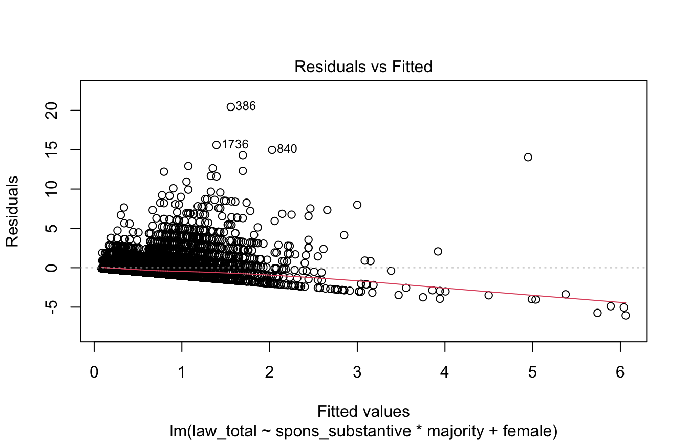
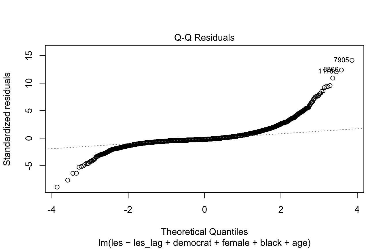
Q-Q Plot
This plot diagnoses non-normality of the residuals.
We want the points to form a diagonal line; if they appear sigmoid or otherwise deviate from the line (especially in the tails) it indicates the residuals are not normally distributed. Non-normal residuals mainly threaten your inference in small samples, so in that case you may want to respecify the model or use methods that don’t assume normality.
# Normal Q-Q Plot
plot(model, 2)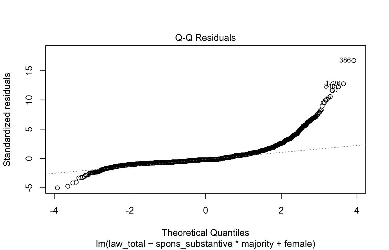
Scale-Location Plot
This plot diagnoses heteroskedasticity.
We want to see a horizontal line and randomly distributed points.
plot(model, 3)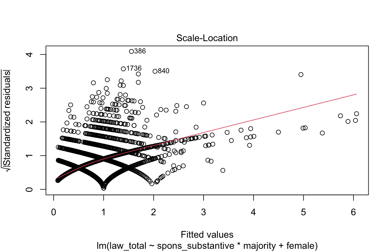
Cook’s Distance
This plot shows whether there are observations that are strongly influencing the fitted values produced by the model. These are often outliers that, when omitted, dramatically change the model estimates.
Generally observations with a Cook’s distance > 0.5 are considered problematic. The below plot labels the observation row numbers with the highest Cook’s distances.
plot(model, 4)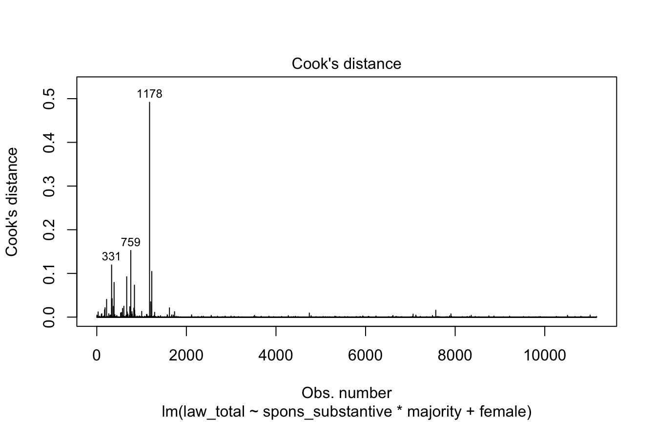
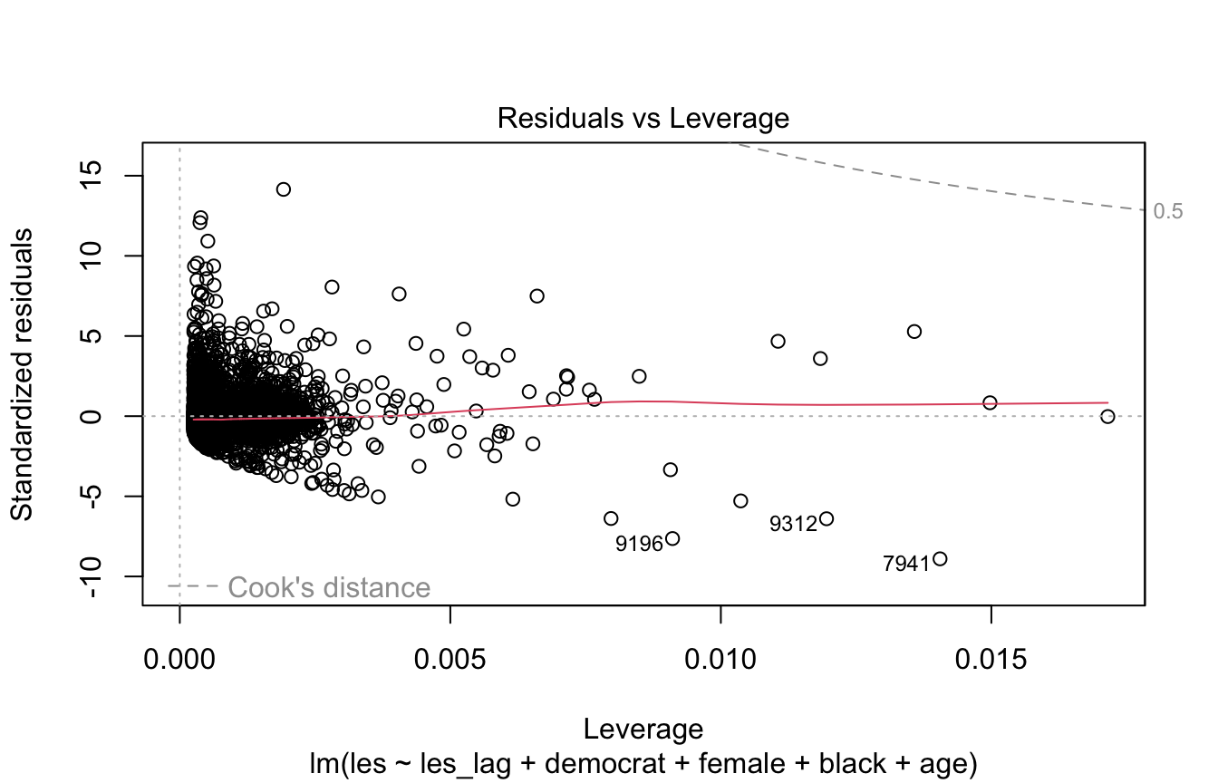
Residuals vs. Leverage
Like Cook’s distance, this plot diagnoses overly-influential observations.
Values beyond the dashed line for 0.5 Cook’s distance are considered overly-influential.
plot(model, 5)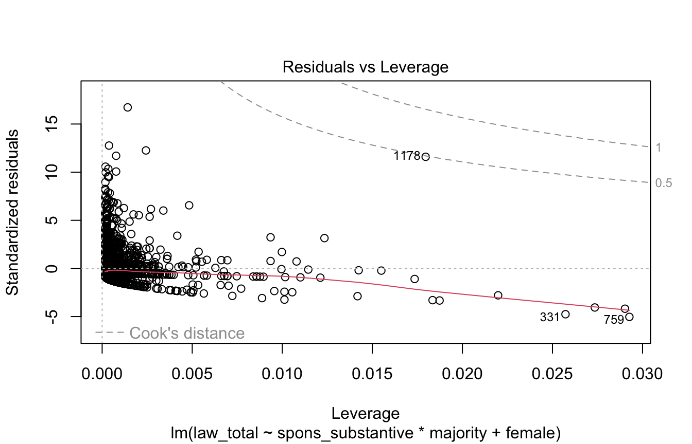
Cook’s Distance vs. Leverage
Similar to Cook’s distance and residuals vs. leverage plot, shows overly-influential observations. Points above a Cook’s distance of 0.5 are problematic.
plot(model, 6)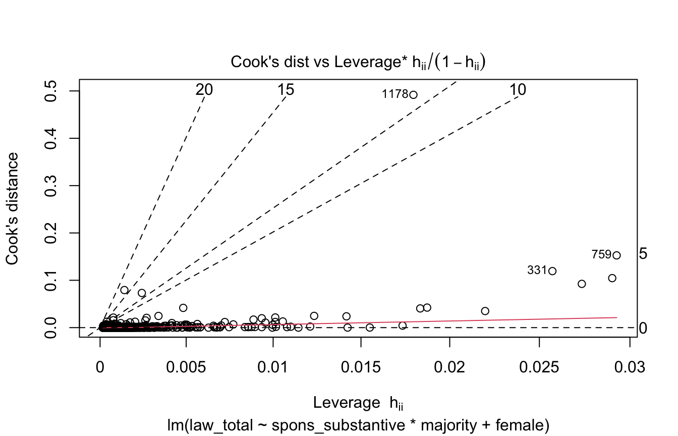
Distribution of Residuals
A basic test of heteroskedasticity/normality of the residuals is to plot them as a histogram or density plot.
If the residuals are normally distributed and centered at zero we’re in good shape.
hist(model$resid)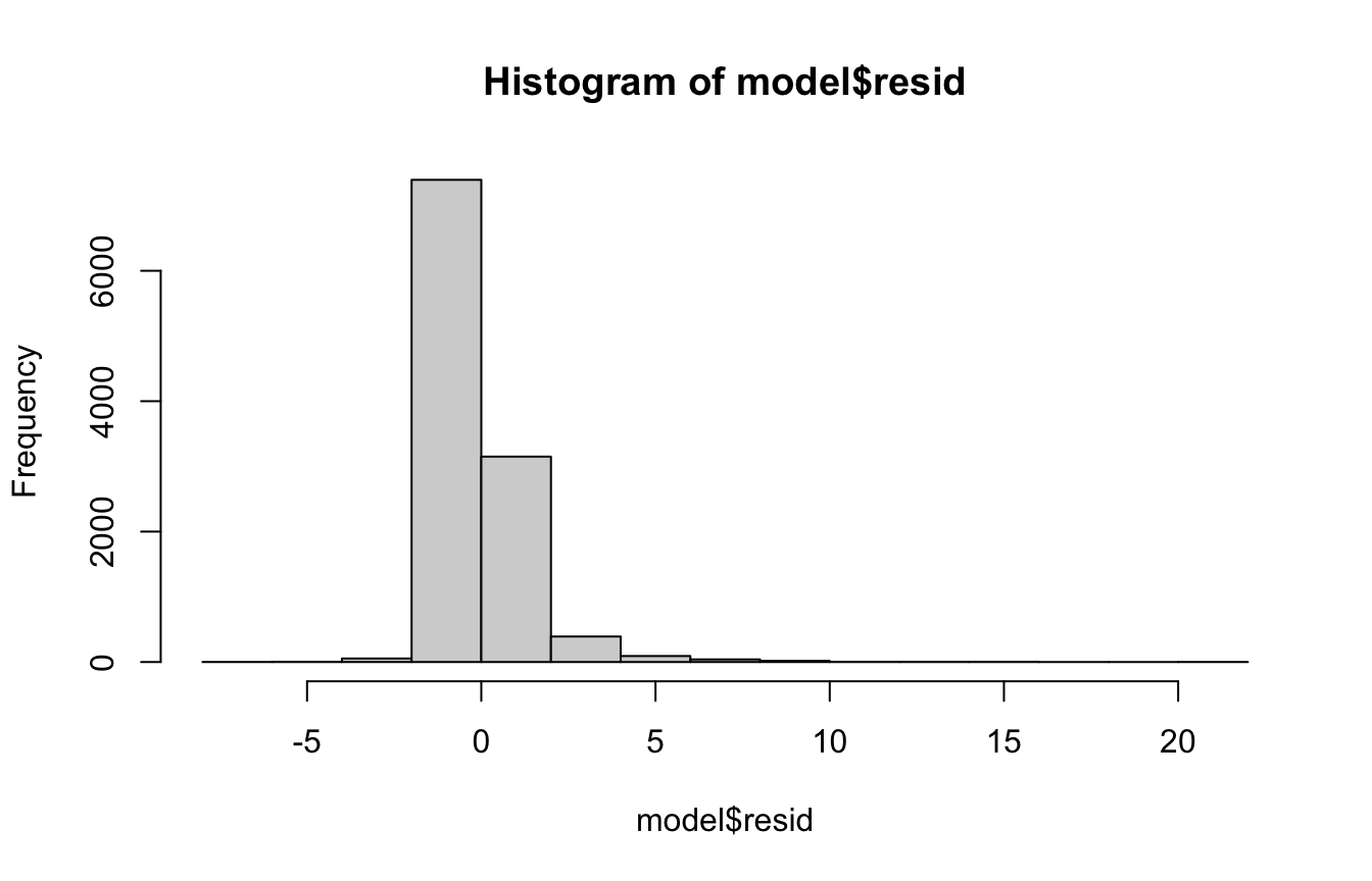
Shapiro-Wilk’s Normality Test
A more concrete test of the normality of the residuals is the Shapiro-Wilk’s normality test. It tests the null hypothesis that the data is normally distributed AKA p<0.05 indicates non-normality.
Note: this test doesn’t work when you have >5,000 observations as in the case below.
#shapiro.test(model$resid) # Doesn't run because n>5,000
shapiro.test(sample(model$resid, 5000))
    Shapiro-Wilk normality test

data:  sample(model$resid, 5000)
W = 0.73641, p-value < 2.2e-16
6.3 Formatting Regression Tables
There are two main libraries used to make publication-quality regression tables:
6.3.1 modelsummary
library(modelsummary)

library(readxl)
CEL <- read_excel("CELHouse.xls")

m1 <- lm(law_total ~ spons_substantive*majority + female, data=CEL)
m2 <- lm(law_total ~ spons_substantive + majority + female, data=CEL)

# Table with a single regression
#
# Useful arguments:
#   output: sets output type, can be set to a number of different kinds
#     of tables, filetypes. See ?modelsummary for more info.
#   stars: when TRUE shows significance stars (this is FALSE by default)
#   vcov: use a different kind of standard errors
#   note: adds text at the bottom of the table
#   coef_rename: lets you rename the coefficients
#   coef_map: lets you rename and omit coefficients
#   gof_omit: omit goodness of fit statistics
#   fmt: control the exact format of coefficients, i.e. # of digits
modelsummary(m1, output="kableExtra", title="Regression table",
             stars=T, notes="This is a note",
             vcov="HC3",
             coef_map=c(spons_substantive="Substantive bills sponsored",
                        majority="Majority party",
                        female="Female",
                        "spons_substantive:majority"="Substantive*majority"),
gof_omit="AIC|BIC") # omit AIC and BIC| (1) | |
|---|---|
| Substantive bills sponsored | 0.008*** |
| (0.001) | |
| Majority party | 0.361*** |
| (0.042) | |
| Female | −0.158*** |
| (0.033) | |
| Substantive*majority | 0.014*** |
| (0.003) | |
| Num.Obs. | 11158 |
| R2 | 0.107 |
| R2 Adj. | 0.107 |
| Log.Lik. | −18074.916 |
| F | 242.243 |
| RMSE | 1.22 |
| Std.Errors | HC3 |
| + p < 0.1, * p < 0.05, ** p < 0.01, *** p < 0.001 | |
| This is a note |
# Table with multiple regressions

# First put your models into a list, make it a named list if you want the
# column for each model in the table to be labelled

m_list <- list(Interaction=m1, "No interaction"=m2)

modelsummary(m_list, output="kableExtra", title="Regression table",
             stars=T, notes="This is a note",
             coef_map=c(spons_substantive="Substantive bills sponsored",
                        majority="Majority party",
                        female="Female",
                        "spons_substantive:majority"="Substantive*majority"),
gof_omit="AIC|BIC")| Interaction | No interaction | |
|---|---|---|
| Substantive bills sponsored | 0.008*** | 0.017*** |
| (0.001) | (0.001) | |
| Majority party | 0.361*** | 0.565*** |
| (0.033) | (0.024) | |
| Female | −0.158*** | −0.153*** |
| (0.035) | (0.036) | |
| Substantive*majority | 0.014*** | |
| (0.002) | ||
| Num.Obs. | 11158 | 11158 |
| R2 | 0.107 | 0.101 |
| R2 Adj. | 0.107 | 0.101 |
| Log.Lik. | −18074.916 | −18114.047 |
| F | 335.620 | 418.419 |
| RMSE | 1.22 | 1.23 |
| + p < 0.1, * p < 0.05, ** p < 0.01, *** p < 0.001 | ||
| This is a note |
There is currently a bug where using a dark theme in RStudio causes kable tables (one possible output type of modelsummary) to have unreadable text. To fix this you can use an extra kable styling option:
library(tidyverse)
library(kableExtra)
modelsummary(m1, output="kableExtra") %>% kable_paper()| (1) | |
|---|---|
| (Intercept) | 0.242 |
| (0.026) | |
| spons_substantive | 0.008 |
| (0.001) | |
| majority | 0.361 |
| (0.033) | |
| female | −0.158 |
| (0.035) | |
| spons_substantive × majority | 0.014 |
| (0.002) | |
| Num.Obs. | 11158 |
| R2 | 0.107 |
| R2 Adj. | 0.107 |
| AIC | 36161.8 |
| BIC | 36205.8 |
| Log.Lik. | −18074.916 |
| F | 335.620 |
| RMSE | 1.22 |
6.3.2 stargazer
I personally prefer modelsummary but stargazer also works well, it has most of the same customization options offered by modelsummary.
library(stargazer)

library(readxl)
CEL <- read_excel("CELHouse.xls")

m1 <- lm(law_total ~ spons_substantive*majority + female, data=CEL)
m2 <- lm(law_total ~ spons_substantive + majority + female, data=CEL)

stargazer(m1, type="text", title="Another regression table")
Another regression table
======================================================
                               Dependent variable:
                           ---------------------------
                                    law_total
------------------------------------------------------
spons_substantive                   0.008***
                                     (0.001)

majority                            0.361***
                                     (0.033)

female                              -0.158***
                                     (0.035)

spons_substantive:majority          0.014***
                                     (0.002)

Constant                            0.242***
                                     (0.026)

------------------------------------------------------
Observations                         11,158
R2                                    0.107
Adjusted R2                           0.107
Residual Std. Error            1.223 (df = 11153)
F Statistic                335.620*** (df = 4; 11153)
======================================================
Note:                      *p<0.1; **p<0.05; ***p<0.01
6.4 Plotting Results
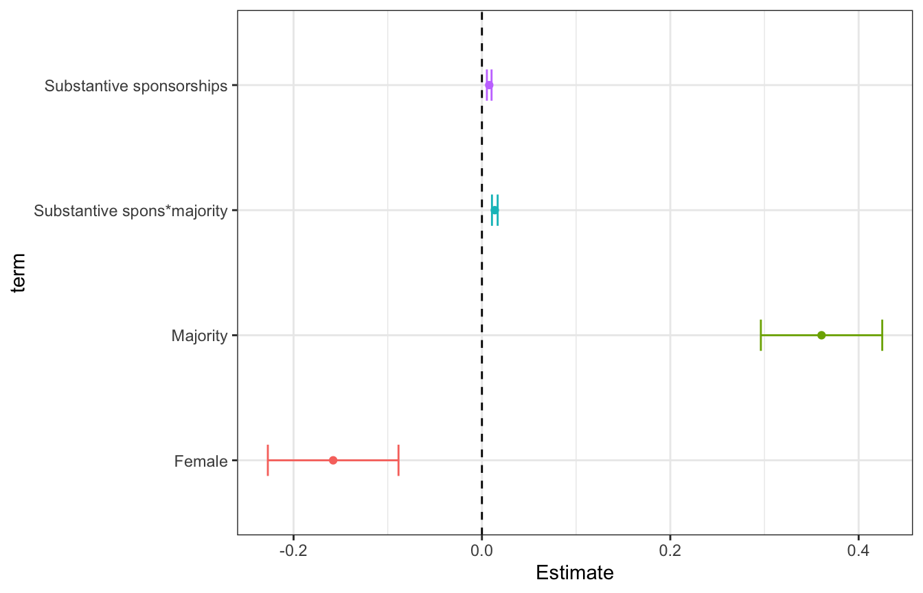
6.4.1 Coefficient Plots
Plots to compare the magnitude of coefficients within or across models
library(tidyverse)
library(readxl)
CEL <- read_excel("CELHouse.xls")

model <- lm(law_total ~ spons_substantive*majority +female,
            data=CEL)

# Coefficient plot two ways:

# Custom plot with ggplot
df_coef_model <- data.frame(coef(summary(model)))
df_coef_model$term <- rownames(df_coef_model) # get a column with our terms

df_coef_model %>%
  filter(term!="(Intercept)") %>%
  mutate(term=case_when( # Recode the terms to look nicer on the plot
    term=="spons_substantive:majority"~"Substantive spons*majority",
    term=="spons_substantive"~"Substantive sponsorships",
    term=="majority"~"Majority",
    term=="female"~"Female",
    T ~ NA_character_
  )) %>%
  ggplot(aes(x=Estimate, y=term, color=term)) +
  geom_point() +
  geom_errorbarh(aes(xmin=Estimate-1.96*Std..Error, xmax=Estimate+1.96*Std..Error), height=0.25) + # adds horizontal error bars
  geom_vline(xintercept=0, lty=2) + # add horizontal line at x=0
  theme_bw() +
  theme(
    legend.position="none"
  )
# If you want the orientation changed add coord_flip() and use geom_errorbar()
df_coef_model %>%
  filter(term!="(Intercept)") %>%
  mutate(term=case_when( # Recode the terms to look nicer on the plot
    term=="spons_substantive:majority"~"Substantive spons*majority",
    term=="spons_substantive"~"Substantive sponsorships",
    term=="majority"~"Majority",
    term=="female"~"Female",
    T ~ NA_character_
  )) %>%
  ggplot(aes(x=Estimate, y=term, color=term)) +
  geom_point() +
  geom_errorbarh(aes(xmin=Estimate-1.96*Std..Error, xmax=Estimate+1.96*Std..Error), height=0.25) + # adds horizontal error bars
  geom_vline(xintercept=0, lty=2) + # add horizontal line at x=0
  theme_bw() +
  theme(
    legend.position="none"
  ) +
  coord_flip()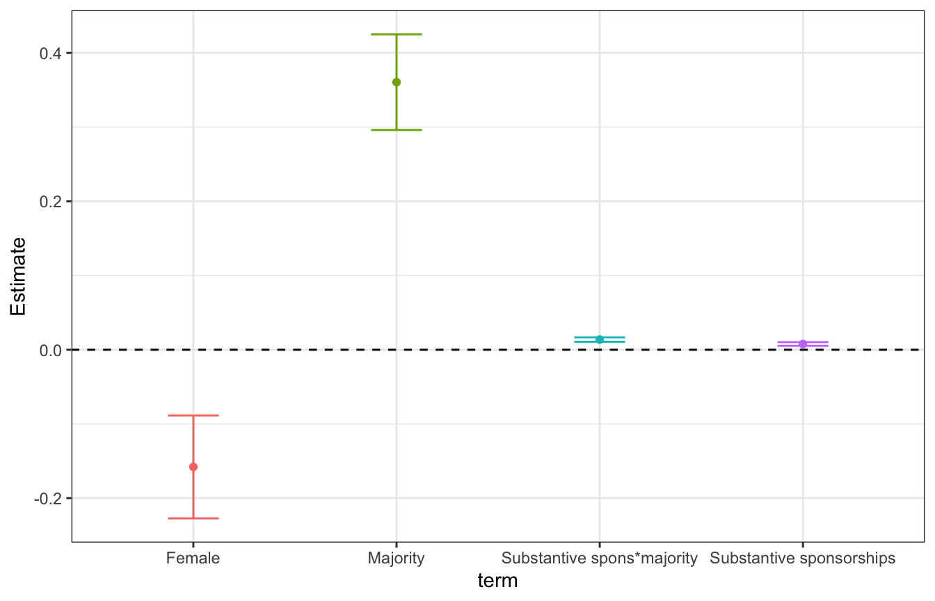
# Using sjPlot
library(sjPlot)

plot_model(model) +
  theme_bw() # Note plot_model uses ggplot so you can add customization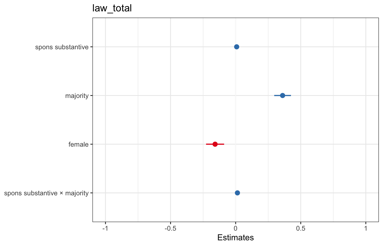
# like you would a regular ggplot6.4.2 Predicted Value Plots
library(sjPlot)

plot_model(model, type="pred", terms=c("spons_substantive"))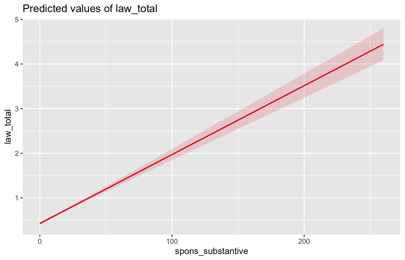
6.4.3 Interaction Plots
library(sjPlot)

plot_model(model, type="int", terms=c("spons_substantive", "majority"))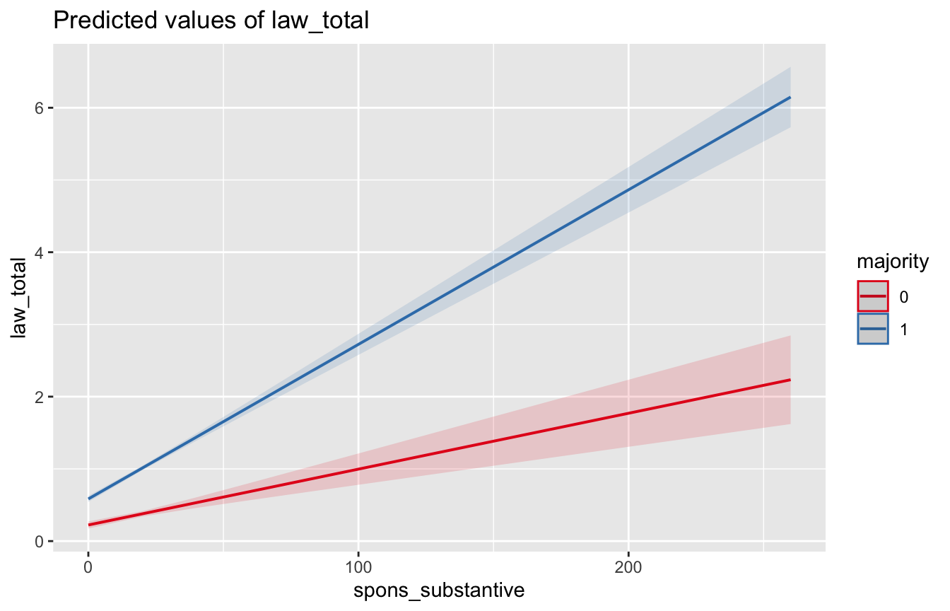
# You can specify values for a scenario like so:
# This plot shows the marginal effect of majority for three values
# of spons_substantive: 0, 100, 200
plot_model(model, type="pred", terms=c("majority","spons_substantive [0,100,200]"))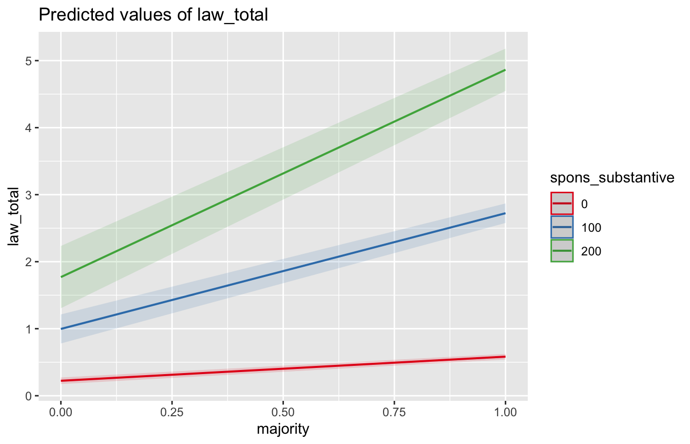
6.5 Standard Errors
library(readxl)
library(tidyverse)
# install.packages("fixest")
library(fixest) # provides fixed effects model estimation and clustered SEs
# install.packages("sandwich")
library(sandwich) # provides robust and clustered SEs for glm
# install.packages("lmtest")
library(lmtest) # provides coeftest() which lets us estimate various kinds of SEs

# Toy data is from the Center for Effective Lawmaking
# Observations are congress-legislator level
# (i.e. Chuck Schumer in the 112th Congress)
df <- read_excel("CELHouse.xls") %>%
  mutate(age=congress_start - year_born)
6.5.1 TLDR
- Regular standard errors are fine when:
- Your errors are homoskedastic, i.e. there’s no reason to think your error might be larger at the extremes of a variable
- Test with:
plot(model)orols_test_breusch_pagan()from theolsrrlibrary
- Test with:
- Your errors wouldn’t be related to some kind of clustering, i.e. if I had reason to think my model would do a worse job making predictions for legislators from Florida I wouldn’t use regular standard errors.
- Your audience isn’t technical/won’t call you out for not using robust standard errors
- Your errors are homoskedastic, i.e. there’s no reason to think your error might be larger at the extremes of a variable
- Robust standard errors are good when:
- Pretty much always, downside is they will be bigger than regular standard errors
- You have reason to believe your errors are heteroskedastic
- Clustered standard errors are good when:
- You expect your errors to be correlated with some sort of clustering variable, especially when your “treatment” is being given at the cluster level
- You’re running a fixed effects model
- Clustered robust standard errors are good when:
- Pretty much always if you were going to use clustered standard errors
- Bootstrapped standard errors are good when:
- You have no other way to estimate standard errors i.e. you’re using some weird nonlinear model
6.5.2 Regular Standard Errors
Baked into lm() and glm()
model <- lm(les ~ les_lag + democrat + female + black + age, data=df)

summary(model)
Call:
lm(formula = les ~ les_lag + democrat + female + black + age,
    data = df)

Residuals:
     Min       1Q   Median       3Q      Max
-11.1072  -0.5128  -0.2748   0.2553  17.7645

Coefficients:
             Estimate Std. Error t value Pr(>|t|)
(Intercept)  0.101476   0.072672   1.396  0.16265
les_lag      0.630093   0.009000  70.007  < 2e-16 ***
democrat     0.089571   0.027915   3.209  0.00134 **
female      -0.059805   0.042573  -1.405  0.16013
black       -0.139162   0.052076  -2.672  0.00755 **
age          0.006112   0.001309   4.669 3.07e-06 ***
---
Signif. codes:  0 '***' 0.001 '**' 0.01 '*' 0.05 '.' 0.1 ' ' 1

Residual standard error: 1.257 on 8862 degrees of freedom
  (2290 observations deleted due to missingness)
Multiple R-squared:  0.3773,    Adjusted R-squared:  0.377
F-statistic:  1074 on 5 and 8862 DF,  p-value: < 2.2e-16
6.5.3 Diagnosing Heteroskedasticity
Looking at some diagnostic plots and running a Breusch Pagan test can help us determine if there is heteroskedasticity
- What we could see in diagnostic plots that could make us worried:
- Residuals vs. fitted: points don’t look like a random cloud
- QQ plot: points not in a straight line
- Scale-location plot: fit is not a horizontal line
- Residuals vs. leverage plot: fit not a horizontal line, particularly want to see if there are values with high leverage and standardized residuals (top right corner of plot)
Breusch-Pagan test will test the null hypothesis that the errors are homoskedastic, AKA if p<.05 we may have heteroskedasticity
# QQ plot not a linear relationship
# Scale location fit is not horizontal
plot(model)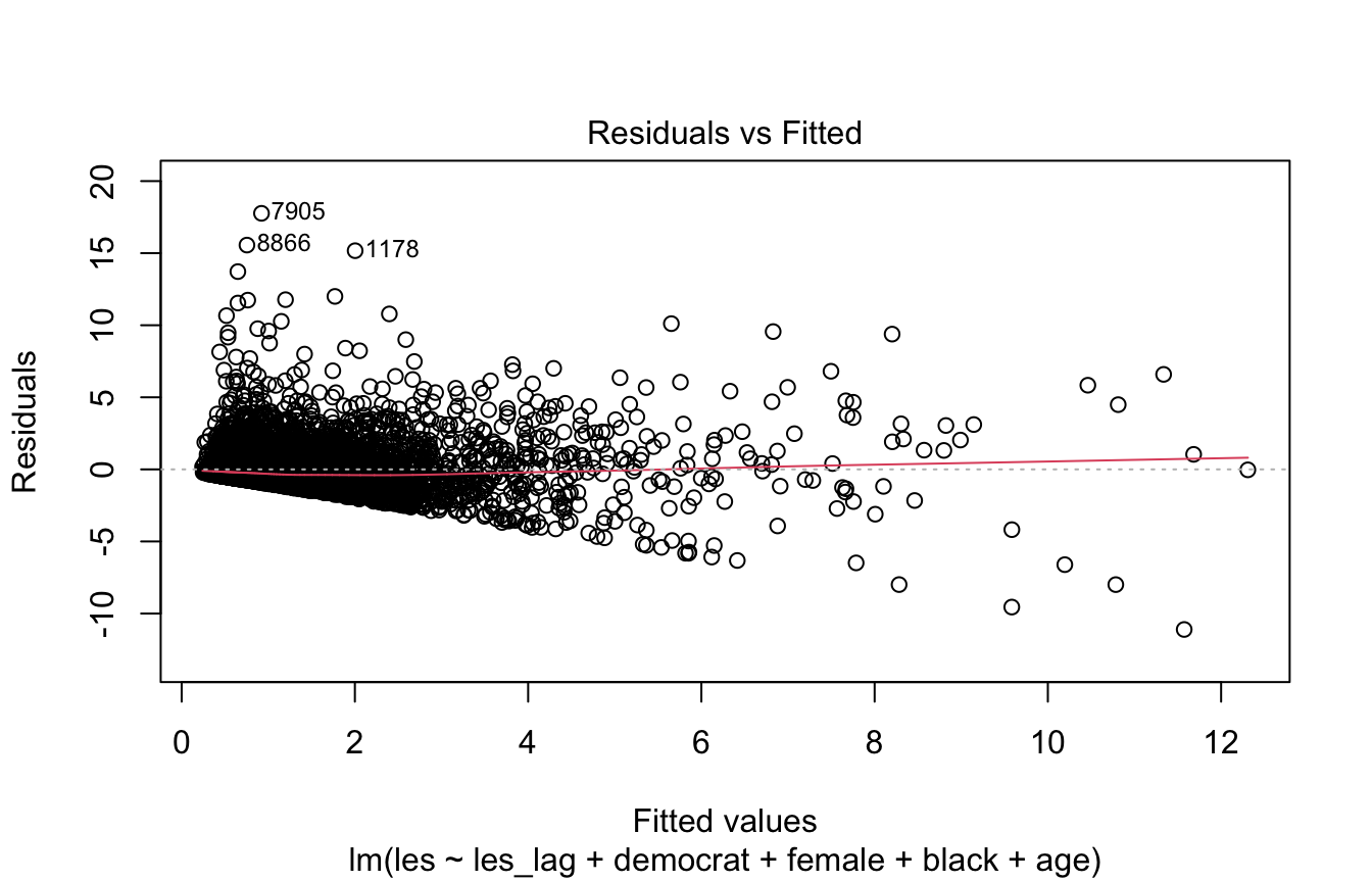
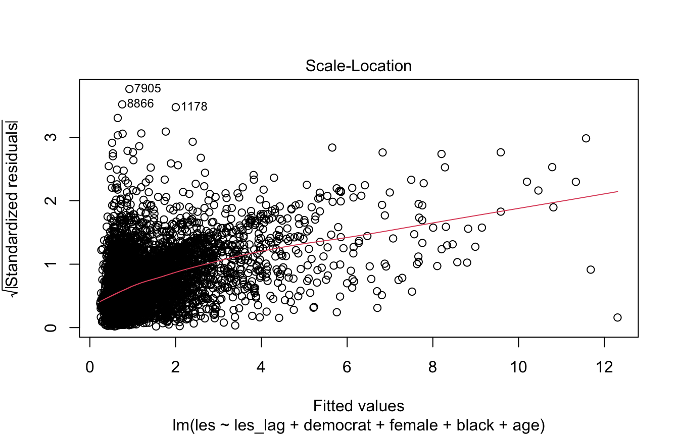
# p < .01 which means we reject the null hypothesis that errors are
# homoskedastic
library(olsrr)
ols_test_breusch_pagan(model)
 Breusch Pagan Test for Heteroskedasticity
 -----------------------------------------
 Ho: the variance is constant
 Ha: the variance is not constant

             Data
 -------------------------------
 Response : les
 Variables: fitted values of les

        Test Summary
 ----------------------------
 DF            =    1
 Chi2          =    7545.6975
 Prob > Chi2   =    0.0000
6.5.4 Robust Standard Errors
coeftest() (from the lmtest library) re-tests a model’s coefficients using a standard-error estimate you supply, rather than the default ones baked into lm()/glm(). You pass it the model plus a vcov argument naming the variance-covariance estimator you want (here, vcovHC for heteroskedasticity-consistent errors) and the specific type. The coefficients themselves don’t change — only their standard errors, t-statistics, and p-values do.
So we’ve established that our errors are likely heteroskedastic–this means we should use robust standard errors.
There are a few kinds of robust (heteroskedasticity-consistent aka HC) standard errors:
(if you wanted to dive deeper this is a good breakdown: https://blog.stata.com/2022/10/06/heteroskedasticity-robust-standard-errors-some-practical-considerations/)
HC0
Honestly, I can’t find anyone saying there’s a scenario where you want to use HC0. It is only unbiased when you have a really large sample, just use HC1 or HC3 instead.
# Note coeftest comes from the lmtest library
# We pass our model, specify we want to do robust errors with vcov=vcovHC,
# and tell it what type of robust errors to estimate
coeftest(model, vcov=vcovHC, type="HC0")
t test of coefficients:

              Estimate Std. Error t value  Pr(>|t|)
(Intercept)  0.1014759  0.0729689  1.3907  0.164359
les_lag      0.6300925  0.0245680 25.6469 < 2.2e-16 ***
democrat     0.0895707  0.0282884  3.1663  0.001549 **
female      -0.0598049  0.0341012 -1.7538  0.079508 .
black       -0.1391617  0.0477802 -2.9125  0.003594 **
age          0.0061120  0.0014247  4.2899 1.806e-05 ***
---
Signif. codes:  0 '***' 0.001 '**' 0.01 '*' 0.05 '.' 0.1 ' ' 1
HC1
These are the default robust standard errors reported by Stata so are often referred to as Stata robust errors.
They’re no good when you have a small sample size and/or a model estimating many coefficients (i.e. when you have few degrees of freedom)–they will underestimate your errors.
If you have a large sample/few regressors they will probably be okay but you’re better off using HC3.
# Note coeftest comes from the lmtest library
# We pass our model, specify we want to do robust errors with vcov=vcovHC,
# and tell it what type of robust errors to estimate
coeftest(model, vcov=vcovHC, type="HC1")
t test of coefficients:

              Estimate Std. Error t value  Pr(>|t|)
(Intercept)  0.1014759  0.0729936  1.3902  0.164502
les_lag      0.6300925  0.0245763 25.6382 < 2.2e-16 ***
democrat     0.0895707  0.0282980  3.1653  0.001555 **
female      -0.0598049  0.0341127 -1.7532  0.079609 .
black       -0.1391617  0.0477964 -2.9116  0.003605 **
age          0.0061120  0.0014252  4.2885 1.818e-05 ***
---
Signif. codes:  0 '***' 0.001 '**' 0.01 '*' 0.05 '.' 0.1 ' ' 1
HC2
Corrects for bias in the variance of the residuals by giving more weight to residuals of observations with high leverage but you should probably just use HC3 instead.
# Note coeftest comes from the lmtest library
# We pass our model, specify we want to do robust errors with vcov=vcovHC,
# and tell it what type of robust errors to estimate
coeftest(model, vcov=vcovHC, type="HC2")
t test of coefficients:

             Estimate Std. Error t value  Pr(>|t|)
(Intercept)  0.101476   0.073019  1.3897  0.164649
les_lag      0.630093   0.024658 25.5529 < 2.2e-16 ***
democrat     0.089571   0.028312  3.1637  0.001563 **
female      -0.059805   0.034127 -1.7524  0.079736 .
black       -0.139162   0.047835 -2.9092  0.003633 **
age          0.006112   0.001426  4.2862 1.836e-05 ***
---
Signif. codes:  0 '***' 0.001 '**' 0.01 '*' 0.05 '.' 0.1 ' ' 1
HC3
Like HC2, corrects for bias in the variance of the residuals by giving more weight to residuals of observations with high leverage but seems to perform better overall than HC2
Generally considered the “safest” option, works well with smaller samples
# Note coeftest comes from the lmtest library
# We pass our model, specify we want to do robust errors with vcov=vcovHC,
# and tell it what type of robust errors to estimate
coeftest(model, vcov=vcovHC, type="HC3")
t test of coefficients:

              Estimate Std. Error t value  Pr(>|t|)
(Intercept)  0.1014759  0.0730692  1.3888  0.164940
les_lag      0.6300925  0.0247493 25.4590 < 2.2e-16 ***
democrat     0.0895707  0.0283349  3.1611  0.001577 **
female      -0.0598049  0.0341530 -1.7511  0.079965 .
black       -0.1391617  0.0478907 -2.9058  0.003672 **
age          0.0061120  0.0014272  4.2825 1.867e-05 ***
---
Signif. codes:  0 '***' 0.001 '**' 0.01 '*' 0.05 '.' 0.1 ' ' 1
Others
There are also HC0m, HC4, HC4m, and HC5 errors but I’ve never seen them used in a social science paper.
6.5.5 Bootstrapped Standard Errors
A couple of reasons we like bootstrapping:
- You don’t have to make any assumptions about distribution of the population you’re studying i.e. it’s non-parametric and super flexible
- It’s pretty easy to do
But downsides are:
- You need a lot of data for it to work properly
- You have to assume taking a sample of n observations from your data is equivalent to taking an n sized sample from the population
The procedure:
- Take a random sample of the data
- Estimate the model with that sample and save the coefficient estimates
- Repeat this n times
- We now have a distribution of estimates for each coefficient, we get the standard deviation of this distribution for each coefficient and these are our standard errors.
# See Boots.Rmd for how this is done without relying on a library

#install.packages("simpleboot")
library(simpleboot)

# Pass our regression model we want bootstrapped SEs for and set R, the number
# of times we want to estimate the model on a subset of data (equivalent to
# n_samples in the manual code above)
model_boot <- lm.boot(model, R=10)

# Note that the SEs are a bit different than above, this is likely a result of
# setting R to a pretty small number, if we did R=1000 for both it would
# probably be pretty similar but it would take a while to run
summary(model_boot)
BOOTSTRAP OF LINEAR MODEL (method = rows)
Original Model Fit
------------------
Call:
lm(formula = les ~ les_lag + democrat + female + black + age,
data = df)
Coefficients:
(Intercept) les_lag democrat female black age
0.101476 0.630093 0.089571 -0.059805 -0.139162 0.006112
Bootstrap SD's:
(Intercept) les_lag democrat female black age
0.065924140 0.032504221 0.021750586 0.034727211 0.055756784 0.001496136 6.5.6 Clustered Standard Errors
Use when you expect your errors to be correlated with some sort of clustering variable. Most commonly we use clustered standard errors when estimating a fixed effects model or if your treatment is assigned at the cluster level.
For example if in our toy model we thought that a legislator’s party was somehow correlated with or determined by the state they’re from we would cluster our errors at the state-level.
# Note coeftest comes from the lmtest library
# We pass our model, specify we want to do clustered errors with vcov=vcovCL,
# and tell it what variable to cluster by
coeftest(model, vcov=vcovCL, cluster=~state)
t test of coefficients:

              Estimate Std. Error t value  Pr(>|t|)
(Intercept)  0.1014759  0.0741021  1.3694 0.1709072
les_lag      0.6300925  0.0178454 35.3084 < 2.2e-16 ***
democrat     0.0895707  0.0248649  3.6023 0.0003172 ***
female      -0.0598049  0.0503057 -1.1888 0.2345383
black       -0.1391617  0.0453603 -3.0679 0.0021620 **
age          0.0061120  0.0011826  5.1681 2.416e-07 ***
---
Signif. codes:  0 '***' 0.001 '**' 0.01 '*' 0.05 '.' 0.1 ' ' 1
# OR
# We can use feols() from the fixest library which is used for fixed effects
# models but if we don't specify fixed effects and designate the cluster we
# get the same error estimates as above
feols(les ~ les_lag + democrat + female + black + age, cluster=~state, data=df)OLS estimation, Dep. Var.: les
Observations: 8,868
Standard-errors: Clustered (state)
Estimate Std. Error t value Pr(>|t|)
(Intercept) 0.101476 0.074102 1.36941 1.7644e-01
les_lag 0.630093 0.017845 35.30843 < 2.2e-16 ***
democrat 0.089571 0.024865 3.60229 6.7858e-04 ***
female -0.059805 0.050306 -1.18883 2.3961e-01
black -0.139162 0.045360 -3.06792 3.3419e-03 **
age 0.006112 0.001183 5.16814 3.3926e-06 ***
---
Signif. codes: 0 '***' 0.001 '**' 0.01 '*' 0.05 '.' 0.1 ' ' 1
RMSE: 1.25643 Adj. R2: 0.3769716.5.7 Clustered Robust Standard Errors
If we have heteroskedasticity and we want to cluster errors then we use these.
HC1 is the most commonly used but when we have a smaller number of clusters HC2 and HC3 will perform better.
# Note coeftest comes from the lmtest library
# We pass our model, specify we want to do clustered errors with vcov=vcovCL,
# specify the clustering variable, and specify the type of
# robust standard errors we want to use
coeftest(model, vcov = vcovCL, cluster = ~state, type="HC1")
t test of coefficients:

              Estimate Std. Error t value  Pr(>|t|)
(Intercept)  0.1014759  0.0741021  1.3694 0.1709072
les_lag      0.6300925  0.0178454 35.3084 < 2.2e-16 ***
democrat     0.0895707  0.0248649  3.6023 0.0003172 ***
female      -0.0598049  0.0503057 -1.1888 0.2345383
black       -0.1391617  0.0453603 -3.0679 0.0021620 **
age          0.0061120  0.0011826  5.1681 2.416e-07 ***
---
Signif. codes:  0 '***' 0.001 '**' 0.01 '*' 0.05 '.' 0.1 ' ' 1
6.5.8 Comparison with Toy Model
Let’s compare all the different standard errors we estimated for our model
se_standard <- summary(model)$coefficients[,2]
se_hc0 <- coeftest(model, vcov=vcovHC, type="HC0")[,2]
se_hc1 <- coeftest(model, vcov=vcovHC, type="HC1")[,2]
se_hc2 <- coeftest(model, vcov=vcovHC, type="HC2")[,2]
se_hc3 <- coeftest(model, vcov=vcovHC, type="HC3")[,2]
se_boot_R5 <- summary(lm.boot(model, R=5))$stdev.params
se_boot_R10 <- summary(lm.boot(model, R=10))$stdev.params
se_cluster <- coeftest(model, vcov=vcovCL, cluster=~state)[,2]
se_cluster_hc1 <- coeftest(model, vcov=vcovCL, cluster=~state, type="HC1")[,2]


se_compare <- bind_rows(se_standard, se_hc0, se_hc1, se_hc2, se_hc3,
                        se_boot_R5, se_boot_R10, se_cluster, se_cluster_hc1)

se_compare$type = c("standard", "HC0", "HC1", "HC2", "HC3", "bootstrap\nR=5",
                    "bootstrap\nR=10", "clustered", "clustered\nrobust HC1")

se_compare %>% pivot_longer(c(-type), values_to = "error_estimate",
                            names_to = "variable") %>%
  ggplot(aes(x=type, y=error_estimate, fill=type)) +
    geom_bar(position="dodge", stat="identity") +
    labs(x="", y="SE estimate") +
    theme_bw() +
    theme(
      axis.text.x = element_text(angle=75, size=7, vjust=1, hjust=1),
      legend.position = "none",
      strip.text = element_text(size=7)
    ) +
    facet_wrap(~variable, ncol=2, strip.position = "right",
               scales="free_y")
6.5.9 Getting Non-regular SEs into a Nice Table
modelsummary is my go-to for this, it lets you use robust standard errors by passing to the vcov argument either a string (e.g. “HC1”, “HC3”) OR the function that calculates the desired type of variance-covariance matrix like we did above for clustered standard errors (but here we do need to pass the name of our model object and the clustering variable directly to the, for example, vcovCL() function).
AFAIK stargazer does not offer this functionality.
#install.packages("modelsummary")
library(modelsummary)

# Getting HC3 robust SEs
modelsummary(model, vcov="HC3")| (1) | |
|---|---|
| (Intercept) | 0.101 |
| (0.073) | |
| les_lag | 0.630 |
| (0.025) | |
| democrat | 0.090 |
| (0.028) | |
| female | -0.060 |
| (0.034) | |
| black | -0.139 |
| (0.048) | |
| age | 0.006 |
| (0.001) | |
| Num.Obs. | 8868 |
| R2 | 0.377 |
| R2 Adj. | 0.377 |
| AIC | 29229.0 |
| BIC | 29278.7 |
| Log.Lik. | -14607.516 |
| RMSE | 1.26 |
| Std.Errors | HC3 |
# OR modelsummary(model, vcov=vcovHC(model, type="HC3"))# Getting clustered SEs
modelsummary(model, vcov=vcovCL(model, cluster=~state))| (1) | |
|---|---|
| (Intercept) | 0.101 |
| (0.074) | |
| les_lag | 0.630 |
| (0.018) | |
| democrat | 0.090 |
| (0.025) | |
| female | -0.060 |
| (0.050) | |
| black | -0.139 |
| (0.045) | |
| age | 0.006 |
| (0.001) | |
| Num.Obs. | 8868 |
| R2 | 0.377 |
| R2 Adj. | 0.377 |
| AIC | 29229.0 |
| BIC | 29278.7 |
| Log.Lik. | -14607.516 |
| RMSE | 1.26 |
| Std.Errors | Custom |
# Getting clustered robust SEs
modelsummary(model, vcov=vcovCL(model, cluster=~state, type="HC3"))| (1) | |
|---|---|
| (Intercept) | 0.101 |
| (0.080) | |
| les_lag | 0.630 |
| (0.019) | |
| democrat | 0.090 |
| (0.026) | |
| female | -0.060 |
| (0.059) | |
| black | -0.139 |
| (0.050) | |
| age | 0.006 |
| (0.001) | |
| Num.Obs. | 8868 |
| R2 | 0.377 |
| R2 Adj. | 0.377 |
| AIC | 29229.0 |
| BIC | 29278.7 |
| Log.Lik. | -14607.516 |
| RMSE | 1.26 |
| Std.Errors | Custom |
7 Bootstrapping
library(tidyverse)

# Reading and cleaning example data
social <- read.csv("social.csv") %>%
  mutate(age=2006-yearofbirth,
         hawthorne=ifelse(messages=="Hawthorne", 1, 0),
         civicduty=ifelse(messages=="Civic Duty", 1, 0),
         neighbors=ifelse(messages=="Neighbors", 1, 0),
         female=ifelse(sex=="female", 1, 0))
7.1 Bootstrapped Standard Errors
7.1.1 Why bother?
A couple of reasons we like bootstrapping: 1. You don’t have to make any assumptions about distribution of the population you’re studying i.e. it’s non-parametric and super flexible 2. It’s pretty easy to do
But downsides are: 1. You need a lot of data for it to work properly 2. You have to assume taking a sample of n observations from your data is equivalent to taking an n sized sample from the population
7.2 Doing it manually
The procedure: 1. Take a random sample of the data, with replacement (sample_size below) 2. Estimate the model with that sample and save the coefficient estimates 3. Repeat this n times (n_samples below) 4. We now have a distribution of estimates for each coefficient, we get the standard deviation of this distribution for each coefficient and these are our standard errors.
# This function takes the following arguments:
#   data = a dataframe with our data
#   formula = a formula object with our regression formula
#   n_x = the number of x variables we have in the model
#   n_samples = the number of times to estimate the model with a random subset
#               of the data
#   sample_size = the number of observations to include in the subset of data
# It returns a list of bootstrapped standard errors
se_boot <- function(data, formula, n_x, n_samples, sample_size){
  # Create a matrix to store the coefficient estimates, each row contains
  # coefficients estimated from a different subset of the data
  # (ncol=n_x+1 because we are also storing the intercept estimate)
  coefs <- matrix(nrow=n_samples, ncol=n_x+1)

  # Loop n_samples times, i.e. how many times we want to re-estimate the model
  for(i in 1:n_samples){
    # Estimate the model with a random subset of the data
    # sample_n is a function from the dplyr package that gives us random
    # rows from a dataframe
    model <- lm(formula, sample_n(data, sample_size, replace=TRUE))

    # Store the coefficient estimates in row i of our matrix
    coefs[i,] <- model$coefficient
  }

  # Use apply to get the std dev of each column in the matrix, i.e. our
  # bootstrapped standard errors
  return(apply(coefs, FUN=sd, MARGIN=2))
}

# Example run
se_boot(social, as.formula("primary2006 ~ age + hhsize + female"), n_x = 3,
        n_samples=10, sample_size=50000)
[1] 8.440096e-03 7.296568e-05 2.330321e-03 3.405536e-037.2.1 Using simpleboot
There are several packages that will do bootstrapping for you, below I use simpleboot (there is also a more generic boot library that may be useful in other scenarios outside of bootstrapping standard errors).
#install.packages("simpleboot")
library(simpleboot)

model <- lm(primary2006 ~ age + hhsize + female, social)

# Pass our regression model we want bootstrapped SEs for and set R, the number
# of times we want to estimate the model on a subset of data (equivalent to
# n_samples in the manual code above)
model_boot <- lm.boot(model, R=10)

# Note that the SEs are a bit different than above, this is likely a result of
# setting R to a pretty small number, if we did R=1000 for both it would
# probably be pretty similar but it would take a while to run
summary(model_boot)
BOOTSTRAP OF LINEAR MODEL (method = rows)
Original Model Fit
------------------
Call:
lm(formula = primary2006 ~ age + hhsize + female, data = social)
Coefficients:
(Intercept) age hhsize female
0.130632 0.004029 -0.006600 -0.009142
Bootstrap SD's:
(Intercept) age hhsize female
4.870663e-03 7.217591e-05 1.049744e-03 1.313245e-03 7.3 K-fold Cross-validation
Note there are lots of ways to do cross-validation but they’re all doing basically the same thing: seeing how much your estimate changes when you change which observations in your dataset you estimate it with.
K-fold is one of the more common approaches so I go through it here, other methods just partition the data in different ways.
K-fold CV works as follows:
Set a number of folds, \(k\), to partition the data into random subsets.
Estimate/train the model on \(k-1\) of the subsets and compare it to the model trained on the one remaining subset (we call this the held-out data)
Repeat with another \(k-1\) subsets now containing the one previously held out.
Repeat until each fold has been left out once
The average difference between the \(k-1\) estimates and the held out subset’s estimates tells us how stable out estimates are across subsets of the data. We can measure this any number of ways but a simple one you could try if implementing this would be variation in the R^2.
Trying to implement this algorithm as a function would be a good exercise to try, I suspect Molly will make you do it in a homework anyways so I’ll just show how it’s done with a pre-existing package:
#install.packages("caret")
library(caret)

# Set some parameters for our cross-validation
# number is our k
train_control <- trainControl(method="cv", number=10)

# Estimate the models
# It gives us a warning because it notices our outcome variable is binary
# and thinks we might be trying to do classification rather than regression
model_cv <- train(primary2006 ~ age + hhsize + female,
                  data=social, method="lm",
                  trControl=train_control)

# R^2 in this context is telling us how well we would expect our model to fit
# new data
# RMSE and MAE (mean absolute error) are slightly different measures of error
# i.e. how much your model changes depending on what data it's estimated with
model_cv
Linear Regression
305866 samples
3 predictor
No pre-processing
Resampling: Cross-Validated (10 fold)
Summary of sample sizes: 275279, 275280, 275279, 275280, 275279, 275280, ...
Resampling results:
RMSE Rsquared MAE
0.4594667 0.01697359 0.4222138
Tuning parameter 'intercept' was held constant at a value of TRUE8 Examples
8.1 Simulating a Data Generating Process
8.1.1 Problem 1
Suppose the number of articles covering a given legislator, \(L\), on a given day, is a random variable modeled by the function:
\[V(i, s, d)=\mathcal{P}(\lambda=|3s-5d-\theta(i)|)\]
where \(\theta(i)\) is also a random variable drawn from the following distribution and rounded to the nearest integer:
\[\theta(i)=\lceil\mathcal{N}(\mu=\log(i), \sigma=\frac{i}{3})\rfloor\]
These are functions of the following variables that we can observe:
- \(i\), an index of the particular day covered
- \(s\), the legislator’s seniority (number of terms served)
- \(d\), the ideological distance between the legislator and the newspaper’s editorial board, let \(d \in [0,1]\) where \(d=0\) indicates they have the same ideology and \(d=1\) indicates they are on opposite ends of the ideological spectrum.
Simulate the number of articles covering the legislator for days 1 to 100 when they have served 3 terms in three scenarios:
- \(d=0\)
- \(d=0.5\)
- \(d=1\)
and then plot the simulated number of articles on each day for the three scenarios.
Solution:
# Create a vector of indexs for the days (i)
days <- 1:100

# Create a vector with our values of d
distances <- c(0,0.5,1)


# Define a function to calculate theta(i)
theta <- function(i){
  return(round(rnorm(n=1, mean=log(i), sd=i/3)))
}

# Define a function to calculate V(i,s,d)
V <- function(i, s, d){
  return(rpois(n=1, lambda=abs(3*s - 5*d - theta(i))))
}

# Allocate a matrix to store simulated data
leg_sim_data <- matrix(NA, nrow=length(days), ncol=length(distances))


# Loop through each scenario (i.e. value of d): 0, 0.5, 1
for(d in 1:length(distances)){

  # Loop through each day: 1, 2, 3, . . . 100
  for(i in days){

    # Calcuate V(i,s,d) and store in the matrix for the corresponding
    # day (i) and scenario (d)
    leg_sim_data[i, d] <- V(i=i, s=3, d=d)

  }
}

# Plot the results for each d
par(mfrow=c(3,1))
plot(days, leg_sim_data[,1], main="d=0")
plot(days, leg_sim_data[,2], main="d=0.5")
plot(days, leg_sim_data[,3], main="d=1")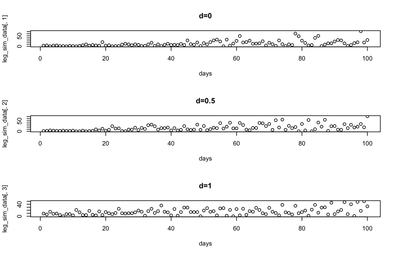
8.1.2 Problem 2
You are trying to model the data generating process behind the decline of local news. Your outcome of interest is \(C_i\), the number of closures of weekly newspapers in state \(i\) in 2019. You suspect \(C_i\) is a function of the following state-level variables:
- \(b_i\), the share of the state’s residents with access to broadband
- \(m_i\), the number of newspaper closures in the state in the previous year
- \(p_i\), the population of the state
- \(g_i\), the state’s GDP in billions of USD
You come up with the following model:
\[C_i(b_i,m_i,p_i,g_i)=\frac{\frac{p_i}{5000}+2\cos{m_i-b_i}}{g_i}\]
Write a custom function,
closures()that takes the above variables as arguments and estimates 2019 newspaper closures for a state using the model above. It should return a single numeric value.Use the
data_problem1defined below to compute an estimate of \(C_i\) for each state.Plot 2019 newspaper closures vs. broadband access.
Hint: no for loops or calls to sapply() are needed to do this.
# Setting seed for reproducibility
set.seed(1234)

# Some simulated data
# Apologies for being too lazy to dig up the actual data
data_problem1 <- data.frame(state=state.name, # R has some built in data like US
                                              # state names
                            broadband=runif(n=50, min=0, max=1),
                            newspaper_closures2018=rpois(n=50, lambda=10),
                            population=runif(n=50, min=581000, max=39000000),
                            GDP=round(runif(n=50, min=40, max=3598)))
Solution:
# Our custom function
closures <- function(b, m, p, g){
  return((p/5000 + 2*cos(m - b))/g)
}

# Calculate our estimates with tidyverse
data_problem1 <- data_problem1 %>%
  mutate(newspaper_closures2019=closures(b=broadband, m=newspaper_closures2018,
                                  p=population, g=GDP))

# or equivalently with base R column operations
# Note we have to call the dataframe each time we access a column unlike
# above in the land of tidyverse
data_problem1$newspaper_closures2019 <- closures(b=data_problem1$broadband,
                                          m=data_problem1$newspaper_closures2018,
                                          p=data_problem1$population,
                                          g=data_problem1$GDP)

# Peek at our data
data_problem1$newspaper_closures2019
[1] 3.2445531 8.5060402 1.3527682 2.7702970 1.7977718 3.7034459 2.3382455
[8] 2.7587508 2.2062562 1.7492582 2.6874203 1.9310147 2.6126009 5.8144861
[15] 15.3012023 2.8117162 2.5493541 61.9474546 0.7887393 4.0693137 1.4674568
[22] 15.6486402 0.7082926 5.9706337 9.5326408 18.2868768 1.8588561 56.6878622
[29] 17.5939514 2.4621804 2.5629531 0.1302537 1.5223657 0.9317214 8.7335019
[36] 2.1479982 2.1207452 1.3675012 4.0695809 3.0942803 4.6081816 2.8546902
[43] 0.2833477 2.2327274 1.6788522 1.6802849 3.5297079 2.3306391 1.5401523
[50] 2.6088156# Plot newspaper closures in 2019 vs. broadband access
plot(x=data_problem1$broadband, y=data_problem1$newspaper_closures2019)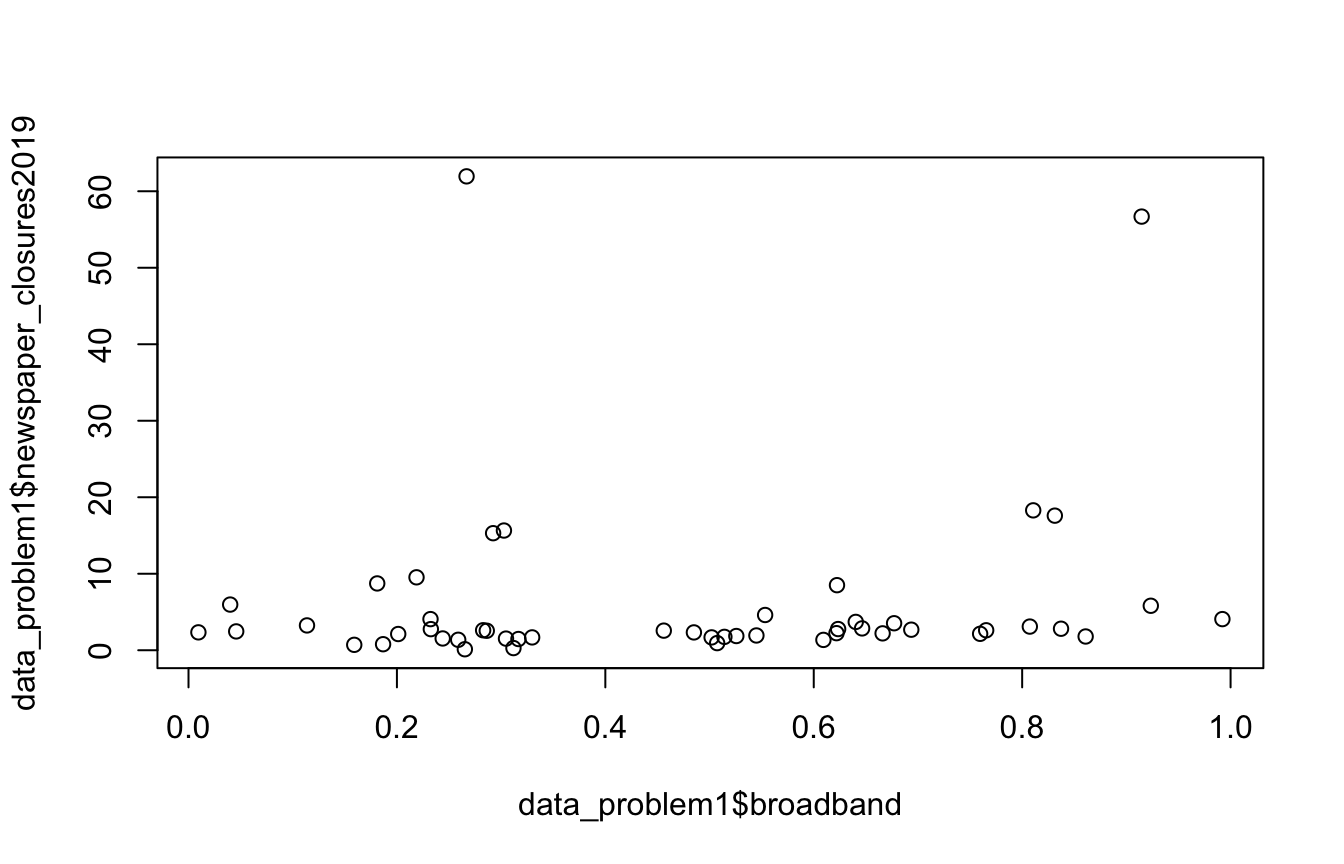
8.2 Writing R Functions
8.2.1 Problem 1
Write a custom function that takes in a vector called vec and an integer int and does the following:
- Reverses the order of the elements in
vecto get a new vectorrev_vec. Hint: You don’t need to do this manually, use a built-in R function. - Multiplies the second half of the elements in
rev_vecbyint. If thevechas an odd length, for example 5, then multiply elements 4 and 5 byint. - Returns
rev_vec
Example input: vec=c(1, 2, 3, 4, 5, 6), int=5 Example output: c(6,5,20,15,10,5)
Solution:
weird_function <- function(vec, int){
  # Reverse the vector
  rev_vec <- rev(vec)

  # Get the length of vec
  l <- length(vec)

  # Get the midpoint of the vector, ceiling() rounds it up if it's odd
  halfway <- ceiling(l/2)

  # Multiply the second half of reversed vector by int
  rev_vec[halfway:l] <- rev_vec[halfway:l]*int

  # Return the modified reversed vector
  return(rev_vec)
}

weird_function(1:6, 5)
[1] 6 5 20 15 10 5Try it yourself. The solution is below — run it, then try your own inputs, or edit the logic and see if you can break it.
8.2.2 Problem 2
Write an expression in R for each of the following mathematical expressions.
For example if given: \(x*y+5\), let \(x=(1,2,3,4,5); y=(2,4,6,8,10)\) You would write in R:
x <- 1:5
y <- seq(from=2,to=10,by=2)

x*y + 5
[1] 7 13 23 37 55Note you may need to use a for loop.
- \(4*[\sum_{i=1}^nx_i^2]+3\), let \(x = (1,2,3,4,5)\)
Correct output: \(223\)
Solution:
x <- 1:5

4*sum(x^2)+3
[1] 223- \(\sum_{i=1}^n x_i^i + y_{2i}\), let \(x=(0,8,5,6); y=(3,6,9,12,15,18,21,24)\)
Correct output: \((6,76,143,1320)\)
Solution:
x <- c(0,8,5,6)
y <- seq(from=3,to=24,by=3)

result <- c()

for(i in 1:length(x)){
  result <- c(result, x[i]^i + y[2*i])
}

sum(result)
[1] 1545- \(\sum_{i=1}^n[\sum_{j=1}^n \ln(x_i/y_j)]\), let \(x=(1,2,3,4,5); y=(2,3,4,5,6,7,8,9)\)
Correct output: -25.7092
Solution:
x <- 1:5
y <- 2:9

result <- 0

for(i in 1:length(x)){
  for(j in 1:length(y)){
    #result <- result + log(x[i]/y[j],base=exp(1))
    result <- result + log(x[i]) - log(y[j])
  }
}

result
[1] -25.70928.2.3 Problem 3
Write a function called problem3 that takes in a vector of strings, vec_strings, and an integer, n. The function does the following:
- Prints the
n-1th element ofvec_strings. - Returns the
nth element ofvec_strings.
You can assume that n will never be larger than the length of vec_strings.
Example input: vec_strings = c("hello", "this", "is", "a", "vector"), n=3 Example output: “this” gets printed, “is” gets returned. The output in console will look like: [1] “this” [1] “is”
Solution:
problem3 <- function(vec_strings, n){
  print(vec_strings[n-1])
  return(vec_strings[n])
}

problem3(c("hello", "this", "is", "a", "vector"), 3)
[1] "this"[1] "is"8.2.4 Problem 4
Write a function called problem4 that takes in a vector of strings, vec_strings, and a vector of integers, vec_ints that are the same length. The function does the following:
- Concatenates each element of
vec_intsto the end of the corresponding element invec_stringsand stores it in a new vector. Hint: you don’t need a for loop to do this part,paste0is your friend. - Sequentially prints each element of this new vector.
- Returns the integer
0.
Example input: vec_strings = c("apple", "pie", "is", "good"), vec_ints = c(4, 3, 1, 5) Example output: [1] “apple4” [1] “pie3” [1] “is1” [1] “good5” [1] 0
Solution:
problem4 <- function(vec_strings, vec_ints){
  vec_new <- paste0(vec_strings, vec_ints)

  for(v in vec_new){
    print(v)
  }

  return(0)
}

problem4(c("apple", "pie", "is", "good"), c(4, 3, 1, 5))
[1] "apple4"
[1] "pie3"
[1] "is1"
[1] "good5"[1] 08.2.5 Problem 5
Write a function called problem5 that takes a vector of integers, vec_ints, an integer, n, and a string, mode. The function does the following:
- If
mode = "modular", each element ofvec_intsis modularly divided bynand this new vector is returned. Hint: to perform modular division we use%%. For example4 %% 2gives0. - If
mode = "normal", each element ofvec_intsis divided bynand this new vector is returned. - If
modeis equal to anything else, return the string “Error: mode incorrectly specified.”.
Example input 1: vec_ints = c(1, 2, 3, 4), n = 2, mode = "modular" Example output 1: 1 0 1 0
Example input 2: vec_ints = c(4, 5, 6, 7, 8, 9, 10), n = 3, mode = "normal" Example output 2: 1.333333 1.666667 2.000000 2.333333 2.666667 3.000000 3.333333
Example input 3: vec_ints = c(10, 11, 12, 13), n = 4, mode = "whatever" Example output 3: “Error: mode incorrectly specified.”
Solution:
problem5 <- function(vec_ints, n, mode){
  if(mode=="modular") return(vec_ints %% n)
  else if(mode=="normal") return(vec_ints / n)
  else return("Error: mode incorrectly specified.")
}

problem5(1:4, 2, "modular")
[1] 1 0 1 0problem5(4:10, 3, "normal")[1] 1.333333 1.666667 2.000000 2.333333 2.666667 3.000000 3.333333problem5(10:13, 4, "whatever")[1] "Error: mode incorrectly specified."8.2.6 Problem 6
Write a function called problem6 that takes in a data frame, df, and an integer, n. The function does the following:
- Checks if
dfhas fewer than 3 columns, if it does then it returns the integer0. - If it has 3 or more columns it subsets
dfto rows 1 ton, i.e. ifn = 3you should subsetdfto have only rows 1, 2, and 3. You can assumenwill always be less than or equal to the number of rows indf. - Returns a vector containing the sum of each column in the subset of
dfyou created in step b. Hint: there is a base R function that will give you the sum of each column.
Example input 1: df = data.frame(x=c(1:5), y=c(6:10)), n = 3 Example output 1: 0
Example input 2: df = data.frame(x=c(1:5), y=c(6:10), z=c(11:15)), n = 2 Example output 2: x y z 3 13 23
Solution:
problem6 <- function(df, n){
  if(ncol(df) < 3) return(0)
  else{
    df <- df[1:n,]
    return(colSums(df))
  }
}

problem6(data.frame(x=c(1:5), y=c(6:10)), 3)
[1] 0problem6(data.frame(x=c(1:5), y=c(6:10), z=c(11:15)), 2) x y z
3 13 23 8.2.7 Problem 7
Write a function called problem7 that takes in two vectors, x and y and does the following:
- Checks if
xandyare the same length, if they aren’t return the integer0. - If
xandyare the same length, it puts them into a new data frame calleddf. - Using ggplot makes the following plots and stores them in the following variables (you can store ggplot plot “objects” with a variable just as you would any other number, string, etc. with the assignment operator
<-):
- A histogram of
xstored ashist_x. - A density plot of
ystored asdens_y. - A scatter plot of
yvs.xstored asscatter_xy.
- These three plots are then stored in a list called
plot_listwhich is returned by the function.
Example input 1: x=1:10, y=100:200 Example output 1: 0
Example input 2: x=1:100, y=(1:100 + runif(100, min=10, max=50)) Example output 2: Console output (it’s printing the list but it contains ggplot objects that can’t be printed in console): [[1]]
[[2]]
[[3]]
Other output: You should see the three plots you made output below the code chunk.
Solution:
problem7 <- function(x, y){
  if(length(x) != length(y)) return(0)
  else{
    library(tidyverse)
    df <- data.frame(x,y)

    hist_x <- ggplot(data=df, aes(x=x)) +
      geom_histogram()

    dens_y <- ggplot(data=df, aes(x=y)) +
      geom_density()

    scatter_xy <- ggplot(data=df, aes(x=x, y=y)) +
      geom_point()

    plot_list <- list(hist_x, dens_y, scatter_xy)

    return(plot_list)
  }
}

problem7(x=1:10, y=100:200)
[1] 0problem7(x=1:100, y=(1:100 + runif(100, min=10, max=50)))[[1]]
[[2]]
[[3]]